clustering

Figure 6. Conceptual similarity between points .

discuss several pragmatic issues associated with its use in Section 5.

5. CLUSTERING TECHNIQUES

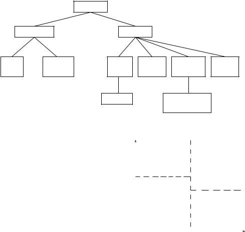
Different approaches to clustering data can be described with the help of the hierarchy shown in Figure 7 (other taxonometric representations of clustering methodology are possible; ours is based on the discussion in Jain and Dubes [1988]). At the top level, there is a distinction between hierarchical and partitional approaches (hierarchical methods produce a nested series of partitions, while partitional methods produce only one).

The taxonomy shown in Figure 7 must be supplemented by a discussion of cross-cutting issues that may (in principle) affect all of the different approaches regardless of their placement in the taxonomy.

ÐAgglomerative vs. divisive: This aspect relates to algorithmic structure and operation. An agglomerative approach begins with each pattern in a distinct (singleton) cluster, and successively merges clusters together until a stopping criterion is satisfied. A divisive method begins with all patterns in a single cluster and performs splitting until a stopping criterion is met.

ÐMonothetic vs. polythetic: This aspect relates to the sequential or simultaneous use of features in the clustering process. Most algorithms are polythetic; that is, all features enter into the computation of distances between patterns, and decisions are based on those distances. A simple monothetic algorithm reported in Anderberg [1973] considers features sequentially to divide the given collection of patterns. This is illustrated in Figure 8. Here, the collection is divided into

two groups using feature x1; the vertical broken line V is the separating line. Each of these clusters is further divided independently using feature

x2, as depicted by the broken lines H1 and H2. The major problem with this algorithm is that it generates 2d clusters where d is the dimensionality of the patterns. For large values of d

(d . 100 is typical in information retrieval applications [Salton 1991]), the number of clusters generated by this algorithm is so large that the data set is divided into uninterestingly small and fragmented clusters.

ÐHard vs. fuzzy: A hard clustering algorithm allocates each pattern to a single cluster during its operation and in its output. A fuzzy clustering method assigns degrees of membership in several clusters to each input pattern. A fuzzy clustering can be converted to a hard clustering by assigning each pattern to the cluster with the largest measure of membership.

ÐDeterministic vs. stochastic: This issue is most relevant to partitional approaches designed to optimize a squared error function. This optimization can be accomplished using traditional techniques or through a random search of the state space consisting of all possible labelings.

ÐIncremental vs. non-incremental: This issue arises when the pattern set

to be clustered is large, and constraints on execution time or memory space affect the architecture of the algorithm. The early history of clustering methodology does not contain many examples of clustering algorithms designed to work with large data sets, but the advent of data mining has fostered the development of clustering algorithms that minimize the number of scans through the pattern set, reduce the number of patterns examined during execution, or reduce the size of data structures used in the algorithm's operations.

A cogent observation in Jain and Dubes [1988] is that the specification of an algorithm for clustering usually leaves considerable flexibilty in implementation.

5.1 Hierarchical Clustering Algorithms

The operation of a hierarchical clustering algorithm is illustrated using the two-dimensional data set in Figure 9. This figure depicts seven patterns labeled A, B, C, D, E, F, and G in three clusters. A hierarchical algorithm yields a dendrogram representing the nested grouping of patterns and similarity levels at which groupings change. A dendrogram corresponding to the seven

Figure 8. Monothetic partitional clustering.

points in Figure 9 (obtained from the single-link algorithm [Jain and Dubes 1988]) is shown in Figure 10. The dendrogram can be broken at different levels to yield different clusterings of the data.

Most hierarchical clustering algorithms are variants of the single-link [Sneath and Sokal 1973], complete-link [King 1967], and minimum-variance [Ward 1963; Murtagh 1984] algorithms. Of these, the single-link and completelink algorithms are most popular. These two algorithms differ in the way they characterize the similarity between a pair of clusters. In the single-link method, the distance between two clus-

X2

F G

Cluster3

Cluster2

Cluster1

C D E

B

A

X1

Figure 9. Points falling in three clusters.

S i m i l a r i t y

A B C D E F G

Figure 10. The dendrogram obtained using the single-link algorithm.

X

Figure 11. Two concentric clusters.

ters is the minimum of the distances between all pairs of patterns drawn from the two clusters (one pattern from the first cluster, the other from the second). In the complete-link algorithm, the distance between two clusters is the maximum of all pairwise distances be-

tween patterns in the two clusters. In either case, two clusters are merged to form a larger cluster based on minimum distance criteria. The complete-link algorithm produces tightly bound or compact clusters [Baeza-Yates 1992]. The single-link algorithm, by contrast, suffers from a chaining effect [Nagy 1968]. It has a tendency to produce clusters that are straggly or elongated. There are two clusters in Figures 12 and 13 separated by a ªbridgeº of noisy patterns. The single-link algorithm produces the clusters shown in Figure 12, whereas the complete-link algorithm obtains the clustering shown in Figure 13. The clusters obtained by the completelink algorithm are more compact than those obtained by the single-link algorithm; the cluster labeled 1 obtained using the single-link algorithm is elongated because of the noisy patterns labeled ª*º. The single-link algorithm is more versatile than the complete-link algorithm, otherwise. For example, the single-link algorithm can extract the concentric clusters shown in Figure 11, but the complete-link algorithm cannot. However, from a pragmatic viewpoint, it has been observed that the completelink algorithm produces more useful hierarchies in many applications than the single-link algorithm [Jain and Dubes 1988].

Agglomerative Single-Link Clustering Algorithm

(1)Place each pattern in its own cluster. Construct a list of interpattern distances for all distinct unordered pairs of patterns, and sort this list in ascending order.

(2)Step through the sorted list of distances, forming for each distinct dis-

similarity value dk a graph on the patterns where pairs of patterns

closer than dk are connected by a graph edge. If all the patterns are members of a connected graph, stop. Otherwise, repeat this step.

X2

X1

Figure 12. A single-link clustering of a pattern set containing two classes (1 and 2) connected by a chain of noisy patterns (*).

Data Clustering · 277

X2

X1

Figure 13. A complete-link clustering of a pattern set containing two classes (1 and 2) connected by a chain of noisy patterns (*).

(3)The output of the algorithm is a nested hierarchy of graphs which can be cut at a desired dissimilarity level forming a partition (clustering) identified by simply connected components in the corresponding graph.

Agglomerative Complete-Link Clustering Algorithm

(1)Place each pattern in its own cluster. Construct a list of interpattern distances for all distinct unordered pairs of patterns, and sort this list in ascending order.

(2)Step through the sorted list of distances, forming for each distinct dis-

similarity value dk a graph on the patterns where pairs of patterns

closer than dk are connected by a graph edge. If all the patterns are members of a completely connected graph, stop.

(3)The output of the algorithm is a nested hierarchy of graphs which can be cut at a desired dissimilarity level forming a partition (clustering) identified by completely connected components in the corresponding graph.

Hierarchical algorithms are more versatile than partitional algorithms. For example, the single-link clustering algorithm works well on data sets containing non-isotropic clusters including

well-separated, chain-like, and concentric clusters, whereas a typical parti-

tional algorithm such as the k-means algorithm works well only on data sets having isotropic clusters [Nagy 1968]. On the other hand, the time and space complexities [Day 1992] of the partitional algorithms are typically lower than those of the hierarchical algorithms. It is possible to develop hybrid algorithms [Murty and Krishna 1980] that exploit the good features of both categories.

Hierarchical Agglomerative Clustering Algorithm

(1)Compute the proximity matrix containing the distance between each pair of patterns. Treat each pattern as a cluster.

(2)Find the most similar pair of clusters using the proximity matrix. Merge these two clusters into one cluster. Update the proximity matrix to reflect this merge operation.

(3)If all patterns are in one cluster, stop. Otherwise, go to step 2.

Based on the way the proximity matrix is updated in step 2, a variety of agglomerative algorithms can be designed. Hierarchical divisive algorithms start with a single cluster of all the given objects and keep splitting the clusters based on some criterion to obtain a partition of singleton clusters.

5.2 Partitional Algorithms

A partitional clustering algorithm obtains a single partition of the data instead of a clustering structure, such as the dendrogram produced by a hierarchical technique. Partitional methods have advantages in applications involving large data sets for which the construction of a dendrogram is computationally prohibitive. A problem accompanying the use of a partitional algorithm is the choice of the number of desired output clusters. A seminal paper [Dubes 1987] provides guidance on this key design decision. The partitional techniques usually produce clusters by optimizing a criterion function defined either locally (on a subset of the patterns) or globally (defined over all of the patterns). Combinatorial search of the set of possible labelings for an optimum value of a criterion is clearly computationally prohibitive. In practice, therefore, the algorithm is typically run multiple times with different starting states, and the best configuration obtained from all of the runs is used as the output clustering.

5.2.1 Squared Error Algorithms. The most intuitive and frequently used criterion function in partitional clustering techniques is the squared error criterion, which tends to work well with isolated and compact clusters. The

squared error for a clustering + of a pattern set - (containing K clusters) is

e2~-, +! 5 OK Onj ix~i j! 2 cji2, j51 i51

where x~i j! is the ith pattern belonging to the jth cluster and cj is the centroid of the jth cluster.

The k-means is the simplest and most commonly used algorithm employing a squared error criterion [McQueen 1967]. It starts with a random initial partition and keeps reassigning the patterns to clusters based on the similarity between the pattern and the cluster centers until

a convergence criterion is met (e.g., there is no reassignment of any pattern from one cluster to another, or the squared error ceases to decrease significantly after some number of iterations).

The k-means algorithm is popular because it is easy to implement, and its

time complexity is O~n!, where n is the number of patterns. A major problem with this algorithm is that it is sensitive to the selection of the initial partition and may converge to a local minimum of the criterion function value if the initial partition is not properly chosen. Figure 14 shows seven two-dimensional patterns. If we start with patterns A, B, and C as the initial means around which the three clusters are built, then we end up with the partition {{A}, {B, C}, {D, E, F, G}} shown by ellipses. The squared error criterion value is much larger for this partition than for the best partition {{A, B, C}, {D, E}, {F, G}} shown by rectangles, which yields the global minimum value of the squared error criterion function for a clustering containing three clusters. The correct three-cluster solution is obtained by choosing, for example, A, D, and F as the initial cluster means.

Squared Error Clustering Method

(1)Select an initial partition of the patterns with a fixed number of clusters and cluster centers.

(2)Assign each pattern to its closest cluster center and compute the new cluster centers as the centroids of the clusters. Repeat this step until convergence is achieved, i.e., until the cluster membership is stable.

(3)Merge and split clusters based on some heuristic information, optionally repeating step 2.

k-Means Clustering Algorithm

(1)Choose k cluster centers to coincide with k randomly-chosen patterns or

k randomly defined points inside the hypervolume containing the pattern set.

Figure 14. The k-means algorithm is sensitive to the initial partition.

(2)Assign each pattern to the closest cluster center.

(3)Recompute the cluster centers using the current cluster memberships.

(4)If a convergence criterion is not met, go to step 2. Typical convergence criteria are: no (or minimal) reassignment of patterns to new cluster centers, or minimal decrease in squared error.

Several variants [Anderberg 1973] of

the k-means algorithm have been reported in the literature. Some of them attempt to select a good initial partition so that the algorithm is more likely to find the global minimum value.

Another variation is to permit splitting and merging of the resulting clusters. Typically, a cluster is split when its variance is above a pre-specified threshold, and two clusters are merged when the distance between their centroids is below another pre-specified threshold. Using this variant, it is possible to obtain the optimal partition starting from any arbitrary initial partition, provided proper threshold values are specified. The well-known ISODATA [Ball and Hall 1965] algorithm employs this technique of merging and splitting clusters. If ISODATA is given the ªellipseº partitioning shown in Figure 14 as an initial partitioning, it will produce the optimal three-cluster parti-

Data Clustering · 279

tioning. ISODATA will first merge the clusters {A} and {B,C} into one cluster because the distance between their centroids is small and then split the cluster {D,E,F,G}, which has a large variance, into two clusters {D,E} and {F,G}.

Another variation of the k-means algorithm involves selecting a different criterion function altogether. The dynamic clustering algorithm (which permits representations other than the centroid for each cluster) was proposed in Diday [1973], and Symon [1977] and describes a dynamic clustering approach obtained by formulating the clustering problem in the framework of maximum-likelihood estimation. The regularized Mahalanobis distance was used in Mao and Jain [1996] to obtain hyperellipsoidal clusters.

5.2.2 Graph-Theoretic Clustering. The best-known graph-theoretic divisive clustering algorithm is based on construction of the minimal spanning tree

(MST) of the data [Zahn 1971], and then deleting the MST edges with the largest lengths to generate clusters. Figure 15 depicts the MST obtained from nine two-dimensional points. By breaking the link labeled CD with a length of 6 units (the edge with the maximum Euclidean length), two clusters ({A, B, C} and {D, E, F, G, H, I}) are obtained. The second cluster can be further divided into two clusters by breaking the edge EF, which has a length of 4.5 units.

The hierarchical approaches are also related to graph-theoretic clustering. Single-link clusters are subgraphs of the minimum spanning tree of the data [Gower and Ross 1969] which are also the connected components [Gotlieb and Kumar 1968]. Complete-link clusters are maximal complete subgraphs, and are related to the node colorability of graphs [Backer and Hubert 1976]. The maximal complete subgraph was considered the strictest definition of a cluster in Augustson and Minker [1970] and Raghavan and Yu [1981]. A graph-ori- ented approach for non-hierarchical structures and overlapping clusters is

X2

E

edge with the maximum length

X1

Figure 15. Using the minimal spanning tree to form clusters.

presented in Ozawa [1985]. The Delaunay graph (DG) is obtained by connecting all the pairs of points that are Voronoi neighbors. The DG contains all the neighborhood information contained in the MST and the relative neighborhood graph (RNG) [Toussaint 1980].

5.3Mixture-Resolving and Mode-Seeking Algorithms

The mixture resolving approach to cluster analysis has been addressed in a number of ways. The underlying assumption is that the patterns to be clustered are drawn from one of several distributions, and the goal is to identify the parameters of each and (perhaps) their number. Most of the work in this area has assumed that the individual components of the mixture density are Gaussian, and in this case the parameters of the individual Gaussians are to be estimated by the procedure. Traditional approaches to this problem involve obtaining (iteratively) a maximum likelihood estimate of the parameter vectors of the component densities [Jain and Dubes 1988].

More recently, the Expectation Maximization (EM) algorithm (a generalpurpose maximum likelihood algorithm [Dempster et al. 1977] for missing-data problems) has been applied to the problem of parameter estimation. A recent book [Mitchell 1997] provides an acces-

sible description of the technique. In the EM framework, the parameters of the component densities are unknown, as are the mixing parameters, and these are estimated from the patterns. The EM procedure begins with an initial estimate of the parameter vector and iteratively rescores the patterns against the mixture density produced by the parameter vector. The rescored patterns are then used to update the parameter estimates. In a clustering context, the scores of the patterns (which essentially measure their likelihood of being drawn from particular components of the mixture) can be viewed as hints at the class of the pattern. Those patterns, placed (by their scores) in a particular component, would therefore be viewed as belonging to the same cluster.

Nonparametric techniques for densi- ty-based clustering have also been developed [Jain and Dubes 1988]. Inspired by the Parzen window approach to nonparametric density estimation, the corresponding clustering procedure searches for bins with large counts in a multidimensional histogram of the input pattern set. Other approaches include the application of another partitional or hierarchical clustering algorithm using a distance measure based on a nonparametric density estimate.

5.4 Nearest Neighbor Clustering

Since proximity plays a key role in our intuitive notion of a cluster, nearestneighbor distances can serve as the basis of clustering procedures. An iterative procedure was proposed in Lu and Fu [1978]; it assigns each unlabeled pattern to the cluster of its nearest labeled neighbor pattern, provided the distance to that labeled neighbor is below a threshold. The process continues until all patterns are labeled or no additional labelings occur. The mutual neighborhood value (described earlier in the context of distance computation) can also be used to grow clusters from near neighbors.

Traditional clustering approaches generate partitions; in a partition, each pattern belongs to one and only one cluster. Hence, the clusters in a hard clustering are disjoint. Fuzzy clustering extends this notion to associate each pattern with every cluster using a membership function [Zadeh 1965]. The output of such algorithms is a clustering, but not a partition. We give a high-level partitional fuzzy clustering algorithm below.

Fuzzy Clustering Algorithm

X

Figure 16. Fuzzy clusters.

selecting the N 3 K membership

matrix U. An element uij of this matrix represents the grade of mem-

bership of object xi in cluster cj. Typically, uij [ @0,1#.

(2)Using U, find the value of a fuzzy criterion function, e.g., a weighted squared error criterion function, associated with the corresponding partition. One possible fuzzy criterion function is

E2~-, U! 5 ON OK uijixi 2 cki2,

i51k51

N

where ck 5 ( uikxi is the kth fuzzy

i51

cluster center.

Reassign patterns to clusters to reduce this criterion function value and recompute U.

(3)Repeat step 2 until entries in U do not change significantly.

In fuzzy clustering, each cluster is a fuzzy set of all the patterns. Figure 16 illustrates the idea. The rectangles enclose two ªhardº clusters in the data:

H1 5 $1,2,3,4,5% and H2 5 $6,7,8,9%. A fuzzy clustering algorithm might pro-

duce the two fuzzy clusters F1 and F2 depicted by ellipses. The patterns will

each cluster. For example, fuzzy cluster F1 could be compactly described as

$~1,0.9!, ~2,0.8!, ~3,0.7!, ~4,0.6!, ~5,0.55!,

~6,0.2!, ~7,0.2!, ~8,0.0!, ~9,0.0!%

and F2 could be described as

$~1,0.0!, ~2,0.0!, ~3,0.0!, ~4,0.1!, ~5,0.15!,

~6,0.4!, ~7,0.35!, ~8,1.0!, ~9,0.9!%

The ordered pairs ~i, mi! in each cluster represent the ith pattern and its mem-

bership value to the cluster mi. Larger membership values indicate higher confidence in the assignment of the pattern to the cluster. A hard clustering can be obtained from a fuzzy partition by thresholding the membership value.

Fuzzy set theory was initially applied to clustering in Ruspini [1969]. The book by Bezdek [1981] is a good source for material on fuzzy clustering. The most popular fuzzy clustering algorithm

is the fuzzy c-means (FCM) algorithm. Even though it is better than the hard

k-means algorithm at avoiding local minima, FCM can still converge to local minima of the squared error criterion. The design of membership functions is the most important problem in fuzzy clustering; different choices include

those based on similarity decomposition and centroids of clusters. A generalization of the FCM algorithm was proposed by Bezdek [1981] through a family of

objective functions. A fuzzy c-shell algorithm and an adaptive variant for detecting circular and elliptical boundaries was presented in Dave [1992].

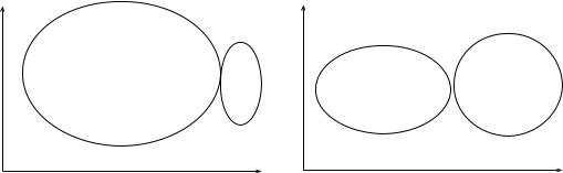
5.6 Representation of Clusters

In applications where the number of classes or clusters in a data set must be discovered, a partition of the data set is the end product. Here, a partition gives an idea about the separability of the data points into clusters and whether it is meaningful to employ a supervised classifier that assumes a given number of classes in the data set. However, in many other applications that involve decision making, the resulting clusters have to be represented or described in a compact form to achieve data abstraction. Even though the construction of a cluster representation is an important step in decision making, it has not been examined closely by researchers. The notion of cluster representation was introduced in Duran and Odell [1974] and was subsequently studied in Diday and Simon [1976] and Michalski et al. [1981]. They suggested the following representation schemes:

(1)Represent a cluster of points by their centroid or by a set of distant points in the cluster. Figure 17 depicts these two ideas.

(2)Represent clusters using nodes in a classification tree. This is illustrated in Figure 18.

(3)Represent clusters by using conjunctive logical expressions. For example,

the expression @X1 . 3#@X2 , 2# in Figure 18 stands for the logical state-

ment `X1 is greater than 3' and 'X2 is less than 2'.

Use of the centroid to represent a cluster is the most popular scheme. It works well when the clusters are compact or isotropic. However, when the clusters are elongated or non-isotropic, then this scheme fails to represent them properly. In such a case, the use of a collection of boundary points in a cluster captures its shape well. The number of points used to represent a cluster should increase as the complexity of its shape increases. The two different representations illustrated in Figure 18 are equivalent. Every path in a classification tree from the root node to a leaf node corresponds to a conjunctive statement. An important limitation of the typical use of the simple conjunctive concept representations is that they can describe only rectangular or isotropic clusters in the feature space.

Data abstraction is useful in decision making because of the following:

(1)It gives a simple and intuitive description of clusters which is easy for human comprehension. In both conceptual clustering [Michalski

and Stepp 1983] and symbolic clustering [Gowda and Diday 1992] this representation is obtained without using an additional step. These algorithms generate the clusters as well as their descriptions. A set of fuzzy rules can be obtained from fuzzy clusters of a data set. These rules can be used to build fuzzy classifiers and fuzzy controllers.

(2)It helps in achieving data compression that can be exploited further by a computer [Murty and Krishna 1980]. Figure 19(a) shows samples belonging to two chain-like clusters labeled 1 and 2. A partitional clus-

tering like the k-means algorithm cannot separate these two structures properly. The single-link algorithm works well on this data, but is computationally expensive. So a hybrid approach may be used to exploit the desirable properties of both these algorithms. We obtain 8 subclusters of the data using the (com-

putationally efficient) k-means algorithm. Each of these subclusters can be represented by their centroids as shown in Figure 19(a). Now the sin- gle-link algorithm can be applied on these centroids alone to cluster them into 2 groups. The resulting groups are shown in Figure 19(b). Here, a data reduction is achieved

by representing the subclusters by their centroids.

(3)It increases the efficiency of the decision making task. In a clusterbased document retrieval technique [Salton 1991], a large collection of documents is clustered and each of the clusters is represented using its centroid. In order to retrieve documents relevant to a query, the query is matched with the cluster centroids rather than with all the documents. This helps in retrieving relevant documents efficiently. Also in several applications involving large data sets, clustering is used to perform indexing, which helps in efficient decision making [Dorai and Jain 1995].

5.7Artificial Neural Networks for Clustering

Artificial neural networks (ANNs) [Hertz et al. 1991] are motivated by biological neural networks. ANNs have been used extensively over the past three decades for both classification and clustering [Sethi and Jain 1991; Jain and Mao 1994]. Some of the features of the ANNs that are important in pattern clustering are: