

clustering
.pdf294 |
· |
A. Jain et al. |
A possible solution to the problem of clustering large data sets while only marginally sacrificing the versatility of clusters is to implement more efficient variants of clustering algorithms. A hybrid approach was used in Ross [1968], where a set of reference points is chosen
as in the k-means algorithm, and each of the remaining data points is assigned to one or more reference points or clusters. Minimal spanning trees (MST) are obtained for each group of points separately. These MSTs are merged to form an approximate global MST. This approach computes similarities between only a fraction of all possible pairs of points. It was shown that the number of similarities computed for 10,000 patterns using this approach is the same as the total number of pairs of points in a collection of 2,000 points. Bentley and Friedman [1978] contains an algorithm that can compute an approximate MST
in O~n log n! time. A scheme to generate an approximate dendrogram incre-
mentally in O~n log n! time was presented in Zupan [1982], while Venkateswarlu and Raju [1992] proposed an algorithm to speed up the ISODATA clustering algorithm. A study of the approximate single-linkage cluster analysis of large data sets was reported in Eddy et al. [1994]. In that work, an approximate MST was used to form sin- gle-link clusters of a data set of size 40,000.
The emerging discipline of data mining (discussed as an application in Section 6) has spurred the development of new algorithms for clustering large data sets. Two algorithms of note are the CLARANS algorithm developed by Ng and Han [1994] and the BIRCH algorithm proposed by Zhang et al. [1996]. CLARANS (Clustering Large Applications based on RANdom Search) identifies candidate cluster centroids through analysis of repeated random samples from the original data. Because of the use of random sampling, the time com-
plexity is O~n! for a pattern set of n elements. The BIRCH algorithm (Bal-
anced Iterative Reducing and Clustering) stores summary information about candidate clusters in a dynamic tree data structure. This tree hierarchically organizes the clusterings represented at the leaf nodes. The tree can be rebuilt when a threshold specifying cluster size is updated manually, or when memory constraints force a change in this threshold. This algorithm, like CLARANS, has a time complexity linear in the number of patterns.
The algorithms discussed above work on large data sets, where it is possible to accommodate the entire pattern set in the main memory. However, there are applications where the entire data set cannot be stored in the main memory because of its size. There are currently three possible approaches to solve this problem.
(1)The pattern set can be stored in a secondary memory and subsets of this data clustered independently, followed by a merging step to yield a clustering of the entire pattern set. We call this approach the divide and conquer approach.
(2)An incremental clustering algorithm can be employed. Here, the entire data matrix is stored in a secondary memory and data items are transferred to the main memory one at a time for clustering. Only the cluster representations are stored in the main memory to alleviate the space limitations.
(3)A parallel implementation of a clustering algorithm may be used. We discuss these approaches in the next three subsections.
5.12.1Divide and Conquer Approach. Here, we store the entire pattern matrix
of size n 3 d in a secondary storage space (e.g., a disk file). We divide this
data into p blocks, where an optimum
value of p can be chosen based on the clustering algorithm used [Murty and Krishna 1980]. Let us assume that we
have n / p patterns in each of the blocks.
ACM Computing Surveys, Vol. 31, No. 3, September 1999
|
|
|
|
|
x |
x |
x |
pk |
|
|
|
|
|
|
|
|
|
|
|
|
|||
|
|
|
|
|
x |
x |
x |
|
|
|
|
|
|
|
|
|
|
|
|
|
|
|
|
|
|
|
|
|
x |
x |
x |
|
|
|
|
x |
x |
x |
x |
|
xxx x |
|
|
x |
x x |
|
|
|
xx x x x |
x x x |
|
x x |
|
|
x x |
x |
x |
n |
|
|
x |
x |
x |
|
|
. . . |
|
x |
|
|
|
|
|
|
|
|
|
-- |
|||||
|
|
x x |
|
|
x |
|
|
x |
|
||
|
|
|
x |
|
|
|
x |
p |
|||
|
|
x x x |
|
x x |
|
|
|
x x |
|
||
|
|
|
|
|
|
|
|
|
|||
|
|
|
|
|
x |
|
|
|
|
|
|
|
|
1 |
|
2 |
|
|
|
p |
|
|
|
Figure 23. |
Divide |
and conquer approach |
to |
||||||||
clustering.
We transfer each of these blocks to the
main memory and cluster it into k clusters using a standard algorithm. One or more representative samples from each of these clusters are stored separately;
we have pk of these representative patterns if we choose one representative
per cluster. These pk representatives
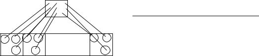
are further clustered into k clusters and the cluster labels of these representative patterns are used to relabel the original pattern matrix. We depict this two-level algorithm in Figure 23. It is possible to extend this algorithm to any number of levels; more levels are required if the data set is very large and the main memory size is very small [Murty and Krishna 1980]. If the singlelink algorithm is used to obtain 5 clusters, then there is a substantial savings in the number of computations as
shown in Table II for optimally chosen p when the number of clusters is fixed at 5. However, this algorithm works well only when the points in each block are reasonably homogeneous which is often satisfied by image data.
A two-level strategy for clustering a data set containing 2,000 patterns was described in Stahl [1986]. In the first level, the data set is loosely clustered into a large number of clusters using the leader algorithm. Representatives from these clusters, one per cluster, are the input to the second level clustering, which is obtained using Ward's hierarchical method.
Data Clustering · 295
Table II. Number of Distance Computations (n) for the Single-Link Clustering Algorithm and a Two-Level Divide and Conquer Algorithm
n |
Single-link |
p |
Two-level |
|
|
|
|
100 |
4,950 |
|
1200 |
500 |
124,750 |
2 |
10,750 |
100 |
499,500 |
4 |
31,500 |
10,000 |
49,995,000 |
10 |
1,013,750 |
|
|
|
|
5.12.2 Incremental Clustering. Incremental clustering is based on the assumption that it is possible to consider patterns one at a time and assign them to existing clusters. Here, a new data item is assigned to a cluster without affecting the existing clusters significantly. A high level description of a typical incremental clustering algorithm is given below.
An Incremental Clustering Algorithm
(1)Assign the first data item to a cluster.
(2)Consider the next data item. Either assign this item to one of the existing clusters or assign it to a new cluster. This assignment is done based on some criterion, e.g. the distance between the new item and the existing cluster centroids.
(3)Repeat step 2 till all the data items are clustered.
The major advantage with the incremental clustering algorithms is that it is not necessary to store the entire pattern matrix in the memory. So, the space requirements of incremental algorithms are very small. Typically, they are noniterative. So their time requirements are also small. There are several incremental clustering algorithms:
(1)The leader clustering algorithm [Hartigan 1975] is the simplest in terms of time complexity which is O~nk!. It has gained popularity because of its neural network implementation, the ART network [Carpenter and Grossberg 1990]. It is very easy to implement as it requires only O~k! space.
ACM Computing Surveys, Vol. 31, No. 3, September 1999
296 |
· |
A. Jain et al. |
(2)The shortest spanning path (SSP) algorithm [Slagle et al. 1975] was originally proposed for data reorganization and was successfully used in automatic auditing of records [Lee et al. 1978]. Here, SSP algorithm was used to cluster 2000 patterns using 18 features. These clusters are used to estimate missing feature values in data items and to identify erroneous feature values.
(3)The cobweb system [Fisher 1987] is an incremental conceptual clustering algorithm. It has been successfully used in engineering applications [Fisher et al. 1993].
(4)An incremental clustering algorithm for dynamic information processing was presented in Can [1993]. The motivation behind this work is that, in dynamic databases, items might get added and deleted over time. These changes should be reflected in the partition generated without significantly affecting the current clusters. This algorithm was used to cluster incrementally an INSPEC database of 12,684 documents corresponding to computer science and electrical engineering.
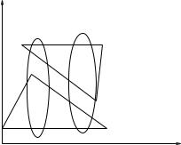
Order-independence is an important property of clustering algorithms. An algorithm is order-independent if it generates the same partition for any order in which the data is presented. Otherwise, it is order-dependent. Most of the incremental algorithms presented above are order-dependent. We illustrate this order-dependent property in Figure 24 where there are 6 two-dimensional objects labeled 1 to 6. If we present these patterns to the leader algorithm in the order 2,1,3,5,4,6 then the two clusters obtained are shown by ellipses. If the order is 1,2,6,4,5,3, then we get a twopartition as shown by the triangles. The SSP algorithm, cobweb, and the algorithm in Can [1993] are all order-depen- dent.
5.12.3 Parallel Implementation. Recent work [Judd et al. 1996] demon-
Y
3 |
4 |
2 |
5 |
|
|
1 |
6 |
X
Figure 24. The leader algorithm is order dependent.
strates that a combination of algorithmic enhancements to a clustering algorithm and distribution of the computations over a network of worksta-
tions can allow an entire 512 3 512 image to be clustered in a few minutes. Depending on the clustering algorithm in use, parallelization of the code and replication of data for efficiency may yield large benefits. However, a global shared data structure, namely the cluster membership table, remains and must be managed centrally or replicated and synchronized periodically. The presence or absence of robust, efficient parallel clustering techniques will determine the success or failure of cluster analysis in large-scale data mining applications in the future.
6. APPLICATIONS
Clustering algorithms have been used in a large variety of applications [Jain and Dubes 1988; Rasmussen 1992; Oehler and Gray 1995; Fisher et al. 1993]. In this section, we describe several applications where clustering has been employed as an essential step. These areas are: (1) image segmentation, (2) object and character recognition, (3) document retrieval, and (4) data mining.
6.1 Image Segmentation Using Clustering
Image segmentation is a fundamental component in many computer vision
ACM Computing Surveys, Vol. 31, No. 3, September 1999
Data Clustering · 297
x3
x2
x1
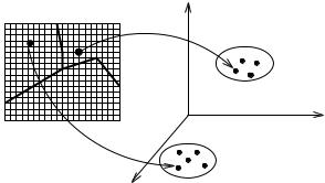
Figure 25. Feature representation for clustering. Image measurements and positions are transformed to features. Clusters in feature space correspond to image segments.
applications, and can be addressed as a clustering problem [Rosenfeld and Kak 1982]. The segmentation of the image(s) presented to an image analysis system is critically dependent on the scene to be sensed, the imaging geometry, configuration, and sensor used to transduce the scene into a digital image, and ultimately the desired output (goal) of the system.
The applicability of clustering methodology to the image segmentation problem was recognized over three decades ago, and the paradigms underlying the initial pioneering efforts are still in use today. A recurring theme is to define feature vectors at every image location (pixel) composed of both functions of image intensity and functions of the pixel location itself. This basic idea, depicted in Figure 25, has been successfully used for intensity images (with or without texture), range (depth) images and multispectral images.
6.1.1 Segmentation. An image segmentation is typically defined as an exhaustive partitioning of an input image into regions, each of which is considered to be homogeneous with respect to some image property of interest (e.g., intensity, color, or texture) [Jain et al. 1995]. If
( 5 $xij, i 5 1. . . Nr, j 5 1. . . Nc%
is the input image with Nr rows and Nc columns and measurement value xij at pixel ~i, j!, then the segmentation can be expressed as 6 5 $S1, . . . Sk%, with the lth segment
Sl 5 $~il1, jl1!, . . . ~ilNl, jlNl!%
consisting of a connected subset of the pixel coordinates. No two segments
share any pixel locations (Si ù Sj 5 À @i Þ j), and the union of all segments
covers |
the |
entire image |
~øik51Si 5 |
$1. . . |
Nr% 3 |
$1. . . Nc%!. |
Jain and |
Dubes [1988], after Fu and Mui [1981] identified three techniques for producing segmentations from input imagery: region-based, edge-based, or clusterbased.
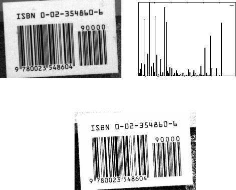
Consider the use of simple gray level thresholding to segment a high-contrast intensity image. Figure 26(a) shows a grayscale image of a textbook's bar code scanned on a flatbed scanner. Part b shows the results of a simple thresholding operation designed to separate the dark and light regions in the bar code area. Binarization steps like this are often performed in character recognition systems. Thresholding in effect `clusters' the image pixels into two groups based on the one-dimensional intensity measurement [Rosenfeld 1969;
ACM Computing Surveys, Vol. 31, No. 3, September 1999
298 |
· |
A. Jain et al. |
’x.dat’
0 50 100 150 200 250 300
(a) (b)
(c)
Figure 26. Binarization via thresholding. (a): Original grayscale image. (b): Gray-level histogram. (c): Results of thresholding.
Dunn et al. 1974]. A postprocessing step separates the classes into connected regions. While simple gray level thresholding is adequate in some carefully controlled image acquisition environments and much research has been devoted to appropriate methods for thresholding [Weszka 1978; Trier and Jain 1995], complex images require more elaborate segmentation techniques.
Many segmenters use measurements which are both spectral (e.g., the multispectral scanner used in remote sensing) and spatial (based on the pixel's location in the image plane). The measurement at each pixel hence corresponds directly to our concept of a pattern.
6.1.2 Image Segmentation Via Clustering. The application of local feature clustering to segment gray±scale images was documented in Schachter et al. [1979]. This paper emphasized the appropriate selection of features at each pixel rather than the clustering methodology, and proposed the use of image plane coordinates (spatial information) as additional features to be employed in clustering-based segmentation. The goal of clustering was to obtain a sequence of hyperellipsoidal clusters starting with cluster centers positioned at maximum density locations in the pattern space, and growing clusters about these cen-
ters until a x2 test for goodness of fit was violated. A variety of features were
ACM Computing Surveys, Vol. 31, No. 3, September 1999
discussed and applied to both grayscale and color imagery.
An agglomerative clustering algorithm was applied in Silverman and Cooper [1988] to the problem of unsupervised learning of clusters of coefficient vectors for two image models that correspond to image segments. The first image model is polynomial for the observed image measurements; the assumption here is that the image is a collection of several adjoining graph surfaces, each a polynomial function of the image plane coordinates, which are sampled on the raster grid to produce the observed image. The algorithm proceeds by obtaining vectors of coefficients
of least-squares fits to the data in M disjoint image windows. An agglomerative clustering algorithm merges (at each step) the two clusters that have a minimum global between-cluster Mahalanobis distance. The same framework was applied to segmentation of textured images, but for such images the polynomial model was inappropriate, and a parameterized Markov Random Field model was assumed instead.
Wu and Leahy [1993] describe the application of the principles of network flow to unsupervised classification, yielding a novel hierarchical algorithm for clustering. In essence, the technique views the unlabeled patterns as nodes in a graph, where the weight of an edge (i.e., its capacity) is a measure of similarity between the corresponding nodes. Clusters are identified by removing edges from the graph to produce connected disjoint subgraphs. In image segmentation, pixels which are 4-neighbors or 8-neighbors in the image plane share edges in the constructed adjacency graph, and the weight of a graph edge is based on the strength of a hypothesized image edge between the pixels involved (this strength is calculated using simple derivative masks). Hence, this segmenter works by finding closed contours in the image, and is best labeled edgebased rather than region-based.
Data Clustering · 299
In Vinod et al. [1994], two neural networks are designed to perform pattern clustering when combined. A twolayer network operates on a multidimensional histogram of the data to identify `prototypes' which are used to classify the input patterns into clusters. These prototypes are fed to the classification network, another two-layer network operating on the histogram of the input data, but are trained to have differing weights from the prototype selection network. In both networks, the histogram of the image is used to weight the contributions of patterns neighboring the one under consideration to the location of prototypes or the ultimate classification; as such, it is likely to be more robust when compared to techniques which assume an underlying parametric density function for the pattern classes. This architecture was tested on gray-scale and color segmentation problems.
Jolion et al. [1991] describe a process for extracting clusters sequentially from the input pattern set by identifying hyperellipsoidal regions (bounded by loci of constant Mahalanobis distance) which contain a specified fraction of the unclassified points in the set. The extracted regions are compared against the best-fitting multivariate Gaussian density through a Kolmogorov-Smirnov test, and the fit quality is used as a figure of merit for selecting the `best' region at each iteration. The process continues until a stopping criterion is satisfied. This procedure was applied to the problems of threshold selection for multithreshold segmentation of intensity imagery and segmentation of range imagery.
Clustering techniques have also been successfully used for the segmentation of range images, which are a popular source of input data for three-dimen- sional object recognition systems [Jain and Flynn 1993]. Range sensors typically return raster images with the measured value at each pixel being the coordinates of a 3D location in space. These 3D positions can be understood
ACM Computing Surveys, Vol. 31, No. 3, September 1999
300 |
· |
A. Jain et al. |
as the locations where rays emerging from the image plane locations in a bundle intersect the objects in front of the sensor.
The local feature clustering concept is particularly attractive for range image segmentation since (unlike intensity measurements) the measurements at each pixel have the same units (length); this would make ad hoc transformations or normalizations of the image features unnecessary if their goal is to impose equal scaling on those features. However, range image segmenters often add additional measurements to the feature space, removing this advantage.
A range image segmentation system described in Hoffman and Jain [1987] employs squared error clustering in a six-dimensional feature space as a source of an ªinitialº segmentation which is refined (typically by merging segments) into the output segmentation. The technique was enhanced in Flynn and Jain [1991] and used in a recent systematic comparison of range image segmenters [Hoover et al. 1996]; as such, it is probably one of the long- est-lived range segmenters which has performed well on a large variety of range images.
This segmenter works as follows. At
each pixel ~i, j! in the input range image, the corresponding 3D measurement
is denoted ~xij, yij, zij!, where typically xij is a linear function of j (the column number) and yij is a linear function of i (the row number). A k 3 k neighborhood of ~i, j! is used to estimate the 3D
surface normal nij 5 ~nxij, nyij, nzij! at ~i, j!, typically by finding the leastsquares planar fit to the 3D points in the neighborhood. The feature vector for
the pixel at ~i, j! is the six-dimensional
measurement ~xij, yij, zij, nxij, nyij, nzij!,
and a candidate segmentation is found by clustering these feature vectors. For practical reasons, not every pixel's feature vector is used in the clustering procedure; typically 1000 feature vectors are chosen by subsampling.
The CLUSTER algorithm [Jain and Dubes 1988] was used to obtain segment labels for each pixel. CLUSTER is
an enhancement of the k-means algorithm; it has the ability to identify several clusterings of a data set, each with a different number of clusters. Hoffman and Jain [1987] also experimented with other clustering techniques (e.g., com- plete-link, single-link, graph-theoretic, and other squared error algorithms) and found CLUSTER to provide the best combination of performance and accuracy. An additional advantage of CLUSTER is that it produces a sequence of output clusterings (i.e., a 2-cluster solu-
tion up through a Kmax-cluster solution
where Kmax is specified by the user and is typically 20 or so); each clustering in this sequence yields a clustering statistic which combines between-cluster separation and within-cluster scatter. The clustering that optimizes this statistic is chosen as the best one. Each pixel in the range image is assigned the segment label of the nearest cluster center. This minimum distance classification step is not guaranteed to produce segments which are connected in the image plane; therefore, a connected components labeling algorithm allocates new labels for disjoint regions that were placed in the same cluster. Subsequent operations include surface type tests, merging of adjacent patches using a test for the presence of crease or jump edges between adjacent segments, and surface parameter estimation.
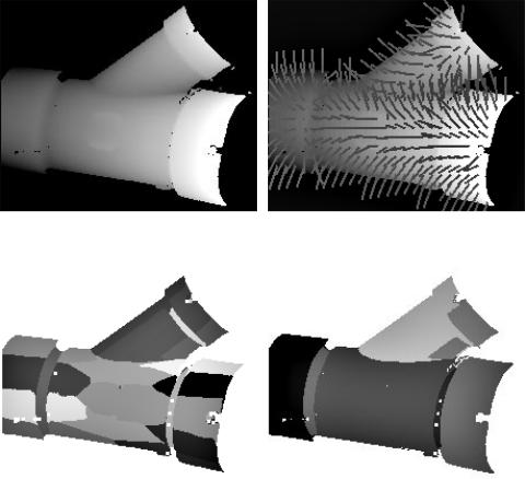
Figure 27 shows this processing applied to a range image. Part a of the figure shows the input range image; part b shows the distribution of surface normals. In part c, the initial segmentation returned by CLUSTER and modified to guarantee connected segments is shown. Part d shows the final segmentation produced by merging adjacent patches which do not have a significant crease edge between them. The final clusters reasonably represent distinct surfaces present in this complex object.
ACM Computing Surveys, Vol. 31, No. 3, September 1999
Data Clustering · 301
(a) |
(b) |
(c) |
(d) |
Figure 27. Range image segmentation using clustering. (a): Input range image. (b): Surface normals for selected image pixels. (c): Initial segmentation (19 cluster solution) returned by CLUSTER using 1000 six-dimensional samples from the image as a pattern set. (d): Final segmentation (8 segments) produced by postprocessing.
The analysis of textured images has been of interest to researchers for several years. Texture segmentation techniques have been developed using a variety of texture models and image operations. In Nguyen and Cohen [1993], texture image segmentation was addressed by modeling the image as a hierarchy of two Markov Random Fields, obtaining some simple statistics from each image block to form a feature vector, and clustering these blocks us-
ing a fuzzy K-means clustering method. The clustering procedure here is modified to jointly estimate the number of
clusters as well as the fuzzy membership of each feature vector to the various clusters.
A system for segmenting texture images was described in Jain and Farrokhnia [1991]; there, Gabor filters were used to obtain a set of 28 orientationand scale-selective features that characterize the texture in the neighborhood of each pixel. These 28 features are reduced to a smaller number through a feature selection procedure, and the resulting features are preprocessed and then clustered using the CLUSTER program. An index statistic
ACM Computing Surveys, Vol. 31, No. 3, September 1999
302 |
· |
A. Jain et al. |
(a) |
(b) |
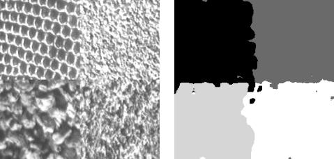
Figure 28. Texture image segmentation results. (a): Four-class texture mosaic. (b): Four-cluster solution produced by CLUSTER with pixel coordinates included in the feature set.
[Dubes 1987] is used to select the best |
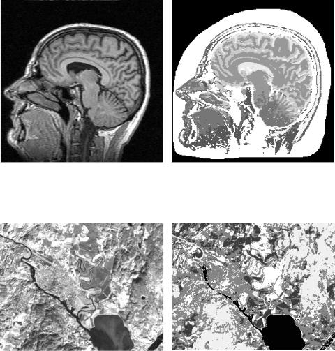
nance imaging channels (yielding a five- |
clustering. Minimum distance classifi- |
dimensional feature vector at each |
cation is used to label each of the origi- |
pixel). A number of clusterings were |
nal image pixels. This technique was |
obtained and combined with domain |
tested on several texture mosaics in- |
knowledge (human expertise) to identify |
cluding the natural Brodatz textures |
the different classes. Decision rules for |
and synthetic images. Figure 28(a) |
supervised classification were based on |
shows an input texture mosaic consist- |
these obtained classes. Figure 29(a) |
ing of four of the popular Brodatz tex- |
shows one channel of an input multi- |
tures [Brodatz 1966]. Part b shows the |
spectral image; part b shows the 9-clus- |
segmentation produced when the Gabor |
ter result. |
filter features are augmented to contain |
The k-means algorithm was applied |
spatial information (pixel coordinates). |
to the segmentation of LANDSAT imag- |
This Gabor filter based technique has |
ery in Solberg et al. [1996]. Initial clus- |
proven very powerful and has been ex- |
ter centers were chosen interactively by |
tended to the automatic segmentation of |
a trained operator, and correspond to |
text in documents [Jain and Bhatta- |
land-use classes such as urban areas, |
charjee 1992] and segmentation of ob- |
soil (vegetation-free) areas, forest, |
jects in complex backgrounds [Jain et |
grassland, and water. Figure 30(a) |
al. 1997]. |
shows the input image rendered as |
Clustering can be used as a prepro- |
grayscale; part b shows the result of the |
cessing stage to identify pattern classes |
clustering procedure. |
for subsequent supervised classifica- |
|
tion. Taxt and Lundervold [1994] and |
6.1.3 Summary. In this section, the |
Lundervold et al. [1996] describe a par- |
application of clustering methodology to |
titional clustering algorithm and a man- |
image segmentation problems has been |
ual labeling technique to identify mate- |
motivated and surveyed. The historical |
rial classes (e.g., cerebrospinal fluid, |
record shows that clustering is a power- |
white matter, striated muscle, tumor) in |
ful tool for obtaining classifications of |
registered images of a human head ob- |
image pixels. Key issues in the design of |
tained at five different magnetic reso- |
any clustering-based segmenter are the |
ACM Computing Surveys, Vol. 31, No. 3, September 1999
Data Clustering · 303
(a) |
(b) |
Figure 29. Multispectral medical image segmentation. (a): A single channel of the input image. (b): 9-cluster segmentation.
(a) |
(b) |
Figure 30. LANDSAT image segmentation. (a): Original image (ESA/EURIMAGE/Sattelitbild). (b): Clustered scene.
choice of pixel measurements (features) and dimensionality of the feature vector (i.e., should the feature vector contain intensities, pixel positions, model parameters, filter outputs?), a measure of similarity which is appropriate for the selected features and the application domain, the identification of a clustering algorithm, the development of strategies for feature and data reduction (to avoid the ªcurse of dimensionalityº and the computational burden of classifying
large numbers of patterns and/or features), and the identification of necessary preand post-processing techniques (e.g., image smoothing and minimum distance classification). The use of clustering for segmentation dates back to the 1960s, and new variations continue to emerge in the literature. Challenges to the more successful use of clustering include the high computational complexity of many clustering algorithms and their incorporation of
ACM Computing Surveys, Vol. 31, No. 3, September 1999