ivchenko_bookreg

2.7.4 Biexcitons and Trions

The existence of biexcitons and charged excitons, or trions, in semiconductors was predicted in 1958 by Lampert [2.122]. These complexes, called originally “excitonic molecule” and “excitonic ion”, are analogous, respectively, to a hydrogen molecule H2 and to an ion H− or ionized molecule H2+. Semiconductor nanostructures allow to realize low-dimensional biexciton and trion states showing the strong increase of the binding energies as compared to the 3D case.

In the e ective mass approximation the biexciton wave function is written

as

where the indices e, h indicate electrons and holes, the indices 1,2 enumerate the identical particles, ϕbiexc is the four-particle envelope function and ψee, ψhh are the Bloch parts. The total wave function has to be antisymmetrical with respect to the exchange of two electrons or two holes. In the biexciton ground state, the electrons and holes form separately spin singlets. This means that the functions ψee, ψhh are antisymmetric, the electronic Bloch part is

and the hole part has a similar form. On the other hand, the ground-state envelope function must be symmetrical to the interchange re1 ↔ re2 or rh1 ↔ rh2. For a QW structure, in the strong-confinement regime, one can use the factored envelope

ϕbiexc = Φ(ρe1, ρe2, ρh2, ρh2) ϕe(ze1) ϕe(ze2) ϕh(zh1) ϕh(zh2) , (2.190)

where the function Φ depends only on the in-plane coordinates, ϕl(zl) is the single-particle quantum-confined function with l = e, h. The envelope Φ satisfies the Schr¨odinger equation with the Hamiltonian

H = − 1 +1 σ 2e1 + 2e2 − 1 +σ σ 2h1 + 2h2

+ 2 (Ve1,h1 + Ve1,h2 + Ve2,h1 + Ve2,h2 + Ve1,e2 + Vh1,h2) ,

where σ is the electron-hole mass ratio me/mh, the units of energy and length are the 3D exciton Rydberg EB and the 3D Bohr radius aB, and the e ective Coulomb interaction is defined by

82 2 Quantum Confinement in Low-Dimensional Systems

Since it is not possible to solve the four-body problem exactly they employ a variational technique. While calculating the biexciton in a single QW structure Kleinman [2.123] chose a trial function

Φ = ξ(β; kρli,l i ) χ(ν, η, λ, τ ; kρh1,h2) ,

χ(ν, η, λ, τ ; ρh1,h2) = uν e−ηu + λe−τ u ,

ξ(β; ρli,l i ) = exp [−(s1 + s2)/2] cosh [β(t1 − t2)/2] ,

containing six variational parameters k, β, ν, η, λ, τ . Here

s1 = ρe1,h1 + ρe1,h2 , s2 = ρe2,h1 + ρe2,h2 ,

t1 = ρe1,h1 − ρe1,h2 , t2 = ρe2,h1 − ρe2,h2 ,

and ρli,l i are the interparticle in-plane distances |ρli − ρl i |. The binding energy εbi of excitons in the biexciton is defined as the di erence

where Eexc and Ebi are the exciton and biexciton excitation energies, accordingly. Calculations show that in the 2D limit εbi exceeds the biexciton binding energy in bulk GaAs by a factor of 3 to 4. An observation of the biexciton state in GaAs/Ga1−xAlxAs QWs was reported in 1982 [2.124]. In II-VI compound semiconductors, it was observed convincingly by B´anyai et al. [2.125]. The further enhancement of the biexiton binding energy is predicted for 1D QWR structures [2.125] and QDs or microcrystallites [2.126]. Multiexciton complexes in InxGa1−xAs/GaAs QDs of the lateral dot sizes

˚

varied around 500 A were investigated in [2.127]. The formation of complexes consisting of three and four excitons becomes possible due to the 3D geometric confinement potential. Their binding energies are negative because the Pauli repulsion pushes additional electrons and holes into higher shells. Binding of two excitons into an excitonic molecule in type-II QW periodic systems is theoretically investigated by Shimura and Matsuura [2.128].

The first identification of charged excitons in a n-doped 2D structure was done by Kheng et al. [2.129]. Since then both the negatively and positively charged trions, X− and X+, composed of two electrons and one hole or two holes and one electron, have been observed and studied in III-V and II-VI 2D systems, see the review [2.130] and references therein. A three-body problem of 2D trions in semiconductor QWs was solved by applying a variational technique [2.131–2.133] or other simplified methods [2.134]. The ground-state wave functions for X− and X+ trions may be written respectively as

= ϕtr,S (ρe1, ρe2, ρh) ϕe(ze1) ϕe(ze2) ϕh(zh) ψee(re1, re2) ψmh0(rh) ,

ΨX+,S

= ϕtr,S (ρe, ρh1, ρh2) ϕe(ze) ϕh(zh1) ϕh(zh2) ψcs0 (re) ψhh(rh1, rh2) .

The negative 2D-trion e ective Hamiltonian measured in units of 2D exciton binding energy, EB2D = 4EB, and 3D exciton Bohr radius is [2.133]

where ρei,h is the distance between the electron i and the hole, ρe1,e2 is the interelectron distance. The similar Hamiltonian for X+ trions is obtained by the change e ↔ h and σ → σ−1. The trion binding energy is defined as

εtr = Eexc − Etr ,

where Eexc, Etr are the exciton and trion excitation energies. A reliable 6-parameter trial function for the singlet state,

is suggested by Sergeev and Suris [2.133]. Here the indices 1, 2 refer to the identical particles, the index 3 refers to the unpaired particle and a, b, c, d, s, R0 are variational parameters. The first multiplier is the symmetrized exciton-like function with di erent orbital radii, the second multiplier accounts for polarization e ects. The parameter d takes into account vibrations of two identical particles around the average distance, R0, between them. The parameter s optimizes the wave function at large distances ρ12.

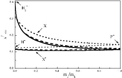
Figure 2.10 shows the calculated trion binding energy, εtr, as a function of the mass ratio σ. Solid, dashed and dotted curves show results of calculation in three di erent approaches. One can see that the binding energy, εtr, of the X− trion is almost independent of σ whereas, for the X+ trion, it remarkably increases with decreasing the mass ratio. At σ → 0, it tends to 0.41.

A simple trial envelope function for the X+ triplet state is [2.135]

It is antisymmetrical with respect to the interchange ρ1 ↔ ρ2 of the hole coordinates. The bound triplet state vanishes as the mass ratio reaches a critical value σcr which, for isotropic e ective masses, is close to 0.35. Near the critical point the triplet binding energy is found from

ε0

εtr ln = A(σ0 − σ) ,

εtr

84 2 Quantum Confinement in Low-Dimensional Systems

Fig. 2.10. Binding energies, εtr, of the X+ and X− 2D-trion singlet states related to the exciton binding energy, εexc, vs. the electron-to-hole mass ratio. Solid and dotted curves are calculated by using the variational method with six [2.133] and twenty two [2.131] fitting parameters. Dashed curve, calculation in a simple analytical model [2.134].

where ε0 ≈ 2.70 and A ≈ 1.17 [2.135].

Excitonic trions in single and double QDs with Gaussian confinement potential were studied by the variational method in [2.136].

2.7.5 Dielectric Response of an Exciton

Here we will derive the relation between the exciton contribution to the dielectric polarization Pexc and the macroscopic electric field E of the light wave. For that we consider the time-dependent wave function |t of the electronic system in the presence of a monochromatic electromagnetic wave of a fixed polarization, α. We assume that the light frequency ω is close to an exciton resonance, ω0, and selection rules allow the resonant photoexcitation only to one excitonic state, |exc, α ≡ |exc , described by the two-particle envelope (2.172). Resonance frequencies of other excitons dipole-active in the same polarization are assumed to be far o enough and their dielectric response as well as that of continuum electron-hole-pair states modified by the Coulomb interaction are taken into account by the background dielectric constant æb. In the linear approximation one has

86 2 Quantum Confinement in Low-Dimensional Systems

Equation (2.202) is also valid for a bulk semiconductor. In this case one

has

where q is the wave vector for the light propagating along z, L is the sample length in this direction. After integration over z and replacement of ϕ1s(0) by (πa3B)−1/2 we obtain

where ωLT is the 3D-exciton longitudinal-transverse splitting,

Equation (2.202) is used in the next chapter in the analysis of resonant light reflection and transmission in QW structures.

3 Resonant Light Reflection and Transmission

Do you send the lightning bolts on their way?

Do they report to you, ‘Here we are’ ?

Job 38: 35

In bulk crystals, a photon and an exciton mix in the dispersion-crossover region, losing their identity in a combined quasi-particle called the exciton polariton. Physically, exciton polaritons can be conveniently considered in terms of an e ective two-oscillator model. The uncoupled photonic and excitonic oscillators are characterized by the same wave vector q and the bare-particle eigenfrequencies

where æb is the background dielectric constant, ω0 is the exciton resonance frequency at q = 0, and M is the exciton e ective mass. The coupling is governed by a value of the exciton longitudinal-transverse splitting, ωLT, and the dispersion equation for coupled excitations can be written as

This is an equivalent form of the conventional dispersion equation

with the one-pole dielectric function

Exciton polaritons were intensively studied in 1960’s and 1970’s, their manifestation in various optical phenomena, including light reflection and transmission, photoluminescence and resonant light scattering, is well-established and documented (see, e.g., the contributed volume [3.1] and references therein). Renewed interest and important developments in this field, see, e.g., [3.2–3.9], were stimulated by technological achievements in fabrication of high-quality nanostructures, multi-layered heterostructures, MQWs, SLs, regular arrays of quantum wires and dots, quantum microcavities. Moreover, the concept of exciton polariton has undergone a substantial modification,

88 3 Resonant Light Reflection and Transmission

in particular with respect to long-period MQW structures containing a fi- nite number of wells [3.10–3.15]. In this chapter, while describing the light reflection and transmission, we will point out the exciton-polariton aspects of these optical processes in various nanostructures.

In short-period heterostructures the interference between “forward-scat- tered” and incident waves is described simply by a macroscopic dielectric function æe (ω) or index of refraction ne = √æe (Sect. 3.1.3). However, such a description is no longer valid for long-period regular structures with the period comparable with the light wavelength λ as shown in Sects. 3.1.2 and 3.1.4. When the QWs are separated by a λ/2, interference between forward and backward waves can strongly attenuate the incident field and enlarge the reflected wave as it occurs in conventional multilayer thin-film dielectric mirrors or distributed Bragg reflectors (Chap. 7). A new and intriguing aspect of the Bragg reflectors is a MQW structure which satisfies the Bragg condition at the exciton resonance frequency, such structures are considered in Sects. 3.1.4 and 3.1.5.

In Sects. 3.1.6 and 3.1.7 we discuss optical properties of QWs grown along directions di erent from [001] and asymmetrical (001)-grown QWs. The electromagnetic response of 0D and 1D structures is described in Sect. 3.2. Electroand magneto-optics in nanostructures are presented in Sects. 3.3 and 3.4, respectively.

3.1 Optical Reflection from Quantum Wells and Superlattices

We will first consider in detail the reflection of light from a single-QW structure and then turn to multiple-QW structures including short-period SLs and resonant Bragg structures.

3.1.1 Single Quantum Well Structure

The amplitude reflection coe cient from the four-layer system ‘vacuum (0) - cap layer (1) - single QW (2) - semiinfinite barrier (3)’ is connected with the coe cient r123 of reflection from the QW by

Here rij (= −rji) and tij are the amplitude coe cients for reflection and transmission of the light falling from a half-infinite medium i (i = 0 in vacuum and i = 1 in layer 1) on the half-infinite medium j, φ1 = q1z d1 is the dephasing due to optical path from the external surface to the interface between the layers 1 and 2, q1z is the z-component of the light wave vector in the layer 1, it is given by

Thus, the problem is reduced to the calculation of the amplitude reflection coe cient r123(ω) for a monochromatic light wave of frequency ω.

ω

ω

ω

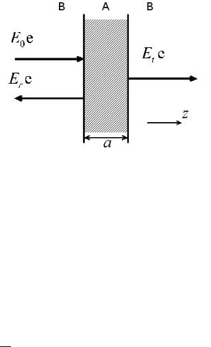
Fig. 3.1. Schematic representation of the normal-incidence light reflection from a single QW.

The problem of light reflection from a single QW neighboring two semiinfinite barrier layers (Fig. 3.1), was solved in 1991 [3.4, 3.5]. The solution has become an important milestone in the development of the quantum electrodynamics studying the coupling between 3D photons and low-dimensional excitons, 2D, 1D or 0D. For simplicity, we assume the normal incidence geometry, θ0 = 0. Then the final result will be reformulated for θ0 = 0. The amplitudes of the electric field for the initial, reflected and transmitted waves are denoted as E0, Er and Et, respectively. For (001)-grown QWs, the three vectors are parallel and we can use the scalar amplitudes E0, Er , Et shown in Fig. 3.1. The electric field outside the QW is given by

(3.7) with q = √æb ω/c. As far as we deal with the linear optics we can omit the factor exp (−iωt). The amplitude reflection and transmission coe cients are