


DENSITY FUNCTIONAL METHOD |
207 |
I3= 122.4 eV
kJ g-1
I2= 75.6 eV
. |
|
. |
I1= 5.4 eV |
. |
|
Fig. 5.16. Caloric equation of state for lithium plasma (Iosilevskii and Gryaznov 1981). The dashed curve is for a pressure of 100 Pa; solid curves are for 0.1 MPa; dashed–dotted curves are for 100 MPa. I1, I2, I3 are the potentials of successive ionization. Other designations are the same as in Fig. 5.15.
1960; Kalitkin and Kuzmina 1975, 1976). The stepwise behavior of the thermodynamic functions in Figs. 5.15 and 5.16 is caused by ionization processes and the steepness of these steps increases as the pressure decreases. The Thomas–Fermi theory, which provides a “smoothed” description of thermodynamic functions, fails to convey peculiarities of the ionization. The characteristic maximum error of the quasiclassical theory in Fig. 5.15 increases and, at ρ → 0, tends to unity. Even more dramatic are the deviations in the caloric equation of state (Fig. 5.16), where the maximum di erence in energy, given by the Saha and Thomas– Fermi approximations in a rarefied plasma, is comparable with the ionization potential per atom and, thus, exceeds substantially the kinetic energy (3/2)kT in the considered limit. Naturally, the deviations in di erential characteristics (heat capacity, compressibility modulus, and so on) will be significant. Analysis by Iosilevskii and Gryaznov (1981) shows that in the limit of full ionization, the internal energy calculated by Kalitkin and Kuzmina (1975, 1976) is shifted relative to the exact value by some constant, which reaches 35–60 % for lithium. Due to the absence of long–range correlations in the cell model, the quasiclassical approximations yield in the caloric equation of state a negative term ρ4/3 corresponding to the nuclear charge interaction with electrons uniformly distributed over the cell volume, instead of giving the Debye term ( ρ3/2).
5.6Density functional method
The method of density functional (MDF) for the energy (thermodynamic potential) is presently the most e ective way of describing strongly interacting dense
208 THERMODYNAMICS OF PLASMAS WITH DEVELOPED IONIZATION
systems. According to the Hohenberg-Kohn theorem and its generalizations, the energy (thermodynamic potential) and wavefunction of the ground state with a nonuniform electron system are single–valued functionals of the distribution of the electron number density ne(r). The consistent use of the MDF to describe the properties of dense electron–ion systems combines simplicity of a quasiclassical method with accurate inclusion of exchange-correlation e ects and bound states. On the other hand, this method is free of considerable mathematical complications associated with the consistent use of the Hartree–Fock method. It is not surprising that the MDF and its modifications were successfully used in various fields of physics to describe the electronic structure of atoms and molecules, clusters, and other small particles, as well as surface phenomena and the properties of solid and liquid metals and nonideal plasma, etc. Also, the MDF is well suited to investigate equations of state of dense systems.
The description of MDF and some of its applications can be found in numerous reviews (see, for example, Lundqvist and March 1983; Rajagopal 1980; Klyuchnikov and Lyubimova 1987). Here, we dwell on the simplest formulation of MDF – a nonuniform electron fluid at T = 0 – and then discuss briefly the calculation of the equation of state for the cell plasma.
The energy of nonuniform electron system in external field V (r) is a functional of its density,
E{ne (r)} = |
V (r) ne (r)dr + |
1 |
|
ne (r) ne(r ) |
drdr + G{ne (r)}. (5.89) |
2 |
|r − r | |
Here G{ne (r)} is the contribution of the kinetic energy and exchange-correlation e ects. The functional G has a universal form, which is not known exactly, so that usually its relatively simple approximations are employed.
Let the electron number density vary slowly, that is, d ln ne(r)/dr kF(r), where kF(r) is the local Fermi wavevector. Then, one can use the gradient expansion of G,
G = |
dr g0 (ne) + g2 (ne) | ne|2 |
+ . . . . |
|
& |
' |
The kinetic and exchange-correlation energies are treated separately by writing
G as the sum G = Ekin + Ee-c. For a degenerate electron gas, |
|
|||||||||
Ekin = |
3 |
3π2 |
! |
2/3 |
|
ne5/3 (r) dr + |
1 |
|
| ne (r)|2ne−1 (r) dr, |
(5.90) |
|
|
|
||||||||
10 |
|
72 |
||||||||
where the second term is the Weizsaecker–Kirzhnitz gradient correction (we use atomic units). A large number of studies have been devoted to the investigation of Ee-c. In a local approximation, one of the simplest expressions for Ee-c is the
interpolation formula of Pines and Nosierez, |
(r) + 0.0474 |
|
||||
Ee-c = − ne (r) |
4 |
π |
ne1/3 |
|
||
|
3 |
3 |
|
1/3 |
|
|
|
+ 0.0155 ln 3π2ne1/3 (r)' dr. |
(5.91) |
||||
DENSITY FUNCTIONAL METHOD |
209 |
The functional (5.89)–(5.91) can be minimized by using a set of trial functions ne(r).
It is interesting that even the simplest approximations, such as (5.89)–(5.91), yield very satisfactory results. For example, the functional given above yields a qualitatively adequate description of the surface properties of alkali metals and even of small metal particles. For small particles, the role of the external potential V (r) is played by the field of the ion core ne(r) = n0θ(R − r), where n0 is the metal density, and R is the particle radius.
By writing the Euler–Lagrange equation for the functional E[ne(r)] and tak-
ing into account conservation ne(r)dr = Ne, one can derive the self–consistent system of Kohn–Sham equations,
|
1 |
|
|
|
|
|
|
||
− |
2 |
2 + Ve (r) ψi (r) = εiψi (r) , |
|
|
(5.92) |
||||
where |
|
|
|
|
|
|
|
|
|
|
|
δE e-c[ne (r)] |
|
n |
(r ) |
||||
Ve (r) = ϕ (r) + |
|
|
|
|
; ϕ (r) = V (r) + |
e |
dr . |
||
|
|
δne (r) |
|
|r − r | |
|||||
The electron number density is given by n lower eigenstates, |
|
|
|||||||
|
|
|
|
|
n |
|
|
|
|
|
|
|
ne (r) = |
|
|ψi (r)|2. |
|
|
(5.93) |
|
|
|
|
|
i |
|
|
|
|
|
|
|
|
|
=1 |
|
|
|
|
|
Therefore, the problem is reduced to the solution of Eq. (5.92), and the self– consistency is provided by (5.95). Unlike the Hartree–Fock equations, the Kohn– Sham equation is exact and the exchange-correlation potential V e-c = δE e-c/δne is local and universal.
The theory is easily generalized to a two–component system at a finite temperature. The free energy F is the functional of the electron and ion distribution,
F = F [ne(r), ni(r)] = f [ne(r), ni(r)]dr.
We restrict ourselves, as above, to the first terms of the gradient expansion and derive,
1 |
|
|
f [ne(r), ni(r)] = g(ne, ni) + |
|
ϕ(ne − ni) + Φa,b na nb, |
2 |
||
|
|
a,b |
where g(ne, ni) is the local free energy density (the quasihomogeneous part of the functional f (ne, ni)), and
ϕ (r) = [ne (r ) − ni (r )]|r − r |−1dr
is the electrostatic potential which satisfies the Poisson equation. In the gradient term, the subscripts a and b stand for e and i.
210 THERMODYNAMICS OF PLASMAS WITH DEVELOPED IONIZATION
Liberman (1979), and Klyuchnikov and Lyubimova (1987) investigated the equation of state for metals in the framework of the cell model. A nucleus shielded by its Z electrons is located at the center of a spherical cavity of radius rs = (3/4πni)−1/3. The distribution of electrons inside the cell is defined by the set of solutions of the Kohn–Sham equation,
2r2 |
|
dr r2 |
drl |
+ |
E − V (r) − l ( |
2r2 |
ul = 0, r rs. |
(5.94) |
|
1 |
|
d |
du |
|
|
|
l + 1) |
|
|
For bound states, the boundary condition is ul(rs) = 0. For free states E = k2/2, the solution of (5.94) should be matched at r = rs with the wavefunction of
ukl(r) cos δl(k)jl(kr) − sin δl(k)nl(kr), r > rs,
where jl and nl are the Bessel and Neumann functions, respectively. The potential V (r) has the form
V (r) = − r |
+ r |
r |
R |
ne (r ) r dr + Ve0-c (ne (r)) , r < rs. |
||
0 |
ne (r ) r 2dr + 4π r |
|||||
|
Z |
|
4π |
|
|
|
The electron distribution is determined similarly to (5.93), but taking into account the weight factors described by the Fermi distribution at given temperature. The solution explicitly divides the electrons into free and bound ones. The pressure of the electron component is equal to that of the Fermi gas of density ne(r) at the spherical boundary of the cell. The ion contribution to the pressure must be calculated separately, which is an independent problem.
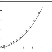
Liberman (1979) calculated the equation of state for cold copper, zinc and nickel. For copper and zinc, this agrees well with the results of dynamic experiments by Altshuler (1965) (see Fig. 5.17). Somewhat worse is the agreement with the measurement results for nickel.
Note the investigations of the thermodynamics of the cell plasma in the Hartree–Fock-Slater approximations (Nikiforov et al. 1979; Sin’ko 1983; Novikov 1985). These methods follow from the MDF. The mentioned papers give results of a broad–range calculations of the equation of state for a number of metals, which are compared with the available experimental data.
5.7Quantum Monte Carlo method
In Section 5.3 we discussed the results of calculations of thermodynamic properties of nonideal plasmas performed with the classical Monte Carlo method. Pair quantum e ects of the electron and ion interactions which caused, in particular, the formation of the bound states at low temperatures, were taken into account approximately in the framework of the pseudopotential model. Recently, the appearance of fast computers and the development of new e cient computational methods stimulated remarkable progress in modeling the thermodynamic
QUANTUM MONTE CARLO METHOD |
211 |
Pa
g cm
Fig. 5.17. Equation of state for zinc at zero temperature: Solid line shows experiment
(Altshuler 1965), points are the calculations (Liberman 1979).
properties with the path–integral Monte Carlo (PIMC) method (Zamalin and Norman 1973; Zamalin, Norman and Filinov 1977; Ceperley 1995; Berne et al. 1998). However, such investigations of the Fermi systems were hampered by the so–called “sign problem”, which was associated with the calculation of sum over all fermion permutations. This eventually resulted in a di erence of two big numbers whose absolute values are practically equal to each other. Ceperley (1995) proposed to overcome this computational obstacle by taking into account only positive terms in the sum, with the simultaneous change of the integration region – the “fixed node approximation”. However, it was not possible to control the computational accuracy with this approximation. One can rigorously prove that this method does not include properly the Fermi statistics, even for an ideal degenerate gas (Filinov 2001). Filinov et al. (2000a,b,c, 2001a,b) have proposed a method to solve the “sign problem”. This method does not involve any approximations and allows us to broaden significantly the range of densities where the simulations can be performed.
The quantum Monte Carlo method is based on direct calculation of the partition function of interacting particles. In the simplest case of a hydrogen plasma, a binary mixture of classical (Boltzmann) Ni protons and Ne quantum electrons is considered. The partition function of such a system can be written as
Z(Ne, Ni, V, β) = Q(Ne, Ni, β)/Ne!Ni!, |
|
||
Q(Ne, Ni, β) = |
σ |
dqdrρ (q, r, σ; β). |
(5.95) |
|
V |
|
|
Here q = {q1, q2, . . . , qNi } are coordinates of the protons, and σ = {σ1, . . . , σNe } and r = {r1, . . . , rNe } are electron spins and coordinates, respectively. The den-
sity matrix ρ in (5.95) is expressed in terms of the path integral,
212 THERMODYNAMICS OF PLASMAS WITH DEVELOPED IONIZATION
ρ (q, r, σ; β) = λi3Ni λ∆3Ne |
P |
(−1)κP |
dr(1) . . . dr(n) × |
||
1 |
|
|
|
|
|
|
|
|
V |
|
|
×ρ q, r, r(1); ∆β |
. . . ρ q, r(n), Pˆr(n+1); ∆β S σ, Pˆσ ,(5.96) |
||||
where ∆β ≡ β/(n + 1), λ2i = 2π 2β/mi, and λ2∆ = 2π 2∆β/me. In Eq. (5.96), r(n+1) ≡ r and σ = σ, i.e., electrons are represented by fermionic loops with
coordinates [r] ≡ +r, r(1), . . . , r(n), r,. The electron spin gives rise to the spin
ˆ
part of the density matrix S, and P is the permutation operator with parity κP . Dimensionless coordinates of quantum electrons are introduced for the calculations and then the density matrix is transformed, so that the sum over the permutations is reduced to the determinant of the exchange matrix ψabn,1,
|
|
|
|
1 |
Ne |
|
|
|
|
|
|
|
|
|
|
|
|
|
|
|
|
|
ρ (q, r, σ; β) = |
|
|
ρs (q, [r], β), |
|
|
|
|||
λ3Ni λ3Ne |
|
|
|
|||||||
σ |
|
i |
∆ |
s=0 |
|
|
|
|
|
|
|
Cs |
|
|
|
n Ne |
|
ψab |
s, |
(5.97) |
|
ρs (q, [r], β) = 2Ne |
exp {−βU (q, [r], β)}l=1 p=1 φpp det |
|||||||||
|
Ne |
|
|
|
- - |
|
|
n,1 |
|
|
|
|
|
|
l |
|
|
|
|
||
|
|
|
n |
e |
ei |
|
|
|
|
|
U (q, [r], β) = U i (q) + |
Ul ([r], β) + Ul |
(q, [r], β) |
. |
|
||||||
|
|
|
||||||||
|
|
l |
|
n + 1 |
|
|
|
|
|
|
|
|
=0 |
|
|
|
|
|
|
|
|
Here U i, Ule, and Ulei are energies of the pair interactions determined by the Kelbg (1964) pseudopotentials between protons, electrons in the lth vertex, as well as between electrons in the lth vertex and protons, respectively. In Eq. (5.97), the
function φppl ≡ exp |
−π ξp(l) |
2 arises from the kinetic part of the density matrix |
|
|
|
|
|
|
presented as a product of high–temperature factors, [r] ≡ [r; r + λ∆ξ(1); r + λ∆(ξ(1) + ξ(2)); . . .], with ξ(1), . . . , ξ(n) being the dimensionless distances between the neighboring vertices on the loop. Components of the exchange matrix ψabn,1 are given by
ψabn,1 |
s ≡ .exp |
−λ∆2 |(ra − rb) + yan|2 |
.s, |
n |
||
yan = λ∆k=1 ξa(k). |
||||||
. . . |
|
π |
. |
|
||
. . . |
|
|
|
. |
|
|
. . . |
|
|
|
. |
|
|
The index s denotes the number of electrons with the same spin projection. Using the determined statistical function, on can derive the total energy and
pressure,
βE = |
3(Ne + Ni) |
− β |
∂ ln Q |
|
βp = |
∂ ln Q |
||
|
|
|
, |
|
. |
|||
2 |
|
∂β |
∂V |
|||||
The standard Metropolis method is applied in order to calculate multiple integrals in such expressions. The accuracy of the results is determined by the
QUANTUM MONTE CARLO METHOD |
213 |
number of factors n in the integrand in Eq. (5.96), the temperature T and the degeneracy parameter χ, via ε (βRy)2χ/(n + 1).
By employing the described method to overcome the “sign problem”, one can describe with high precision thermodynamic properties of an ideal degenerate hydrogen plasma. Filinov et al. (2000a) calculated the pressure versus the degeneracy parameter χ = neλ3e (where λe is the thermal electron wavelength, λ2e = 2π 2β/me) for di erent particle numbers. Even for Ne = 32 the agreement with the analytic dependence was remarkably good up to χ = 10, and it improved as the particle number increased.
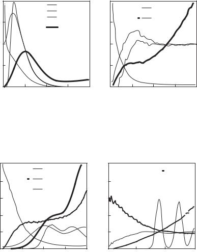
Similar calculations were performed by Filinov et al. (2000b,c) also for nonideal plasmas in a fairly broad range of density, from ne = 1018 to 1026 cm−3, at temperatures from T = 104 to 106 K. In this parameter range di erent phenomena occur, such as partial dissociation and ionization, the Mott transition, and ordering of ions at high densities. The analysis of correlation functions has been performed to investigate these phenomena. Figures 5.18 and 5.19 show the results for four most interesting points in the phase diagram. In Fig. 5.18a at T = 20 000 K and ne = 1022 cm−3, the proton–proton (gii) and electron–electron (gee) correlation functions have sharp maxima at the same coordinate, r = 1.4a0, which suggests that the hydrogen molecules should exist for these conditions. Therefore, in comparison with the Bohr radius a0, the position of the maximum of the electron–proton (gie) correlation function (multiplied by r2) is shifted towards larger values. The molecules disappear as the density decreases, and then a maximum of gie emerges at r = a0. Figure 5.18b shows that the maxima of gii and gee are smeared out as the temperature increases up to T = 50 000 K, which indicates the dissociation of molecules.
The density increase at constant temperature T = 50 000 K results in new physical phenomena. Figures 5.18b and 5.19 clearly demonstrate evolution of the proton–proton correlation function. The curve typical for a partially ionized plasma (see Fig. 5.18b) is modified to that typical for a liquid (Fig. 5.19a) and solid states (Fig. 5.19b).
Also very interesting is the evolution of the electron–electron correlation function as the density grows: The function gee in Fig. 5.18b is typical for partially ionized plasmas, whereas Fig. 5.19a reveals a steep increase at small coordinates. The subsequent density increase results in a more homogeneous electron distribution (see Fig. 5.19b). In order to analyze this phenomenon, the functions r2gee and r2gii are also plotted in Fig. 5.19a. They show that the most probable distance between electrons is two times smaller than that between protons. Analysis of electron trajectories for this case shows pairing of electrons with opposite spins. The “size” of electrons is approximately equal to the distance between protons, which results in partial overlap of the paired electrons.
The region of the hypothetical plasma phase transition is of special interest. To study this phenomenon, the calculations of the hydrogen plasma isotherms at T = 104, 2 · 104, 5 · 104, 105, 1.25 · 105 and 107 K in a broad range of densities from ne = 1018 to 1027 cm−3 were performed by Filinov et al. (2001b). The most
214 THERMODYNAMICS OF PLASMAS WITH DEVELOPED IONIZATION
g(r)
gee gii gei/3
r2gei/10
T = 20 000 K ne = 1022 cm–3
3 |
6 |
9 |
r/a0 |
|
a |
|
|
g(r)
2.0
gei/20
r2gei/30
1.5
1.0
T = 50 000 K
0.5
ne = 1022 cm–3
0 |
2 |
4 |
6 |
r/a0 |
|
|
b |
|
|
Electron–electron (gee, solid line), proton–proton (gii, dashed line) and elec- tron–proton (gie, dashdotted line) pair correlation functions of dense hydrogen plasma. The values for the coupling, degeneracy, and Brueckner parameters are (a) γ = 2.9, χ = 1.46, rs = 5.44 and (b) γ = 1.16, χ = 0.37, rs = 5.44.
|
g(r) |
|
|
|
|
|
5 |
|
gee/4 |
|
|
5 |
|
|
|
|
|
|
||
4 |
|
6r2g |
ee |
|
|
4 |
|
|
|
|
|||
|
|
7r2gii |
|
|
|
|
3 |
T = 50 000 K |
|
|
|
3 |
|
2 |
ne = 5·1025 cm–3 |
|
|
|
2 |
|
|
|
|
|
|
||
1 |
|
|
|
|
|
1 |
0 |
0.2 |
0.4 |
|
0.6 |
0.8 |
0 |
|
|
a |
|
|
r/a0 |
|
|
|
|
|
|
|
|
g(r)
30r2gee
T = 50 000 K ne = 5·1027 cm–3
0.1 0.2 0.3 r/a0
b
Fig. 5.19. Correlation functions of dense hydrogen plasma. The notations are the same as in Fig. 5.18. The values for the coupling, degeneracy, and Brueckner parameters are (a)
γ = 19.8, χ = 1848, rs = 0.318 and (b) γ = 53.8, χ = 37000, rs = 0.117
interesting results are shown in Fig. 5.20 and 5.21.
Figure 5.20 shows the pressure and energy of hydrogen plasma versus density at T = 50 000 K. One can see that the pressure curve (Fig. 5.20a) is monotonic, and the results of this work in good agreement with calculations of Militzer

QUANTUM MONTE CARLO METHOD |
215 |
Pa
. |
. |
. |
. |
. |
. |
g cm |
g cm |
a |
b |
Fig. 5.20. Pressure (a) and energy (b) of a hydrogen plasma vs. density at T = 50 000 K. 1
– direct PIMC simulation (Filinov et al. 2001b), 2 – analytical expression for ideal plasma, 3 – restricted PIMC calculations (Militzer and Ceperley 2001).
and Ceperley (2001) by the quantum Monte Carlo method with restrictions at moderate densities. The curve has a maximum, which suggests formation of bound states.
Another type of behavior is observed as the temperature decreases. Figure 5.21 shows pressure and energy of a hydrogen plasma versus density at T = 10 000 K. Simulations revealed the region of poor convergence to the equilibrium at densities 0.1–1.5 g cm−3, which might suggest the phase transition. Since such anomalies are absent at the T = 50 000 K isotherm, the transition should have a critical point at T 30 000 K. There is a number of additional arguments which make the hypothesis of the phase transition favorable: Calculations with the density functional method performed in the stability region of crystalline hydrogen result in anomalies in the ion–ion correlation function as the density decreases down to ρ = 0.8 g cm−3 (Xu and Hansen 1998) (approximately, the upper density bound for the transition); the maximum density at which the restricted PIMC calculations (Militzer and Ceperley 2001) were possible was ρ = 0.15 g cm−3 (approximately, the lower density bound for the transition); PIMC simulations for a mixture of 33% helium and 67% hydrogen at the same temperature show no transition (curve 3 in Fig. 5.21a); an abrupt increase in the hydrogen electric conductivity (4–5 orders of magnitude) was observed in the shock–wave experiments in a very narrow range of densities, 0.3–0.5 g cm−3, at temperatures 5000–15 000 K (points 6 and 7 in Fig. 5.21a). Finally, in the range of poor convergence at T = 50 000 K and ρ = 0.3346 g cm−3, the visualization of the Monte Carlo cell revealed the formation of proton clusters with the localized electrons, which is a clear indication of the transition to the highly conductive (quasimetallic) state.
In various chemical plasma models (Norman and Starostin 1970; Saumon
216 THERMODYNAMICS OF PLASMAS WITH DEVELOPED IONIZATION
Pa |
Ohm |
cm |
g cm |
g cm |
a |
b |
Fig. 5.21. Pressure and electrical conductivity (a) and energy (b) of a hydrogen plasma vs. density at T = 10 000 K. 1 – direct PIMC simulation (Filinov et al. 2001b), 2 – analytical expression for ideal plasma, 3 – direct PIMC simulation of a mixture consisting of 33% helium and 67% hydrogen (Filinov et al. 2001b), 4 – density functional theory (Xu and Hansen 1998), 5 – restricted PIMC calculations (Militzer and Ceperley 2001), 6 and 7 – experimentally measured electrical conductivity, (Weir et al. 1996) and (Ternovoi et al.
1999), respectively.
and Chabrier 1992), the plasma phase transition occurs approximately at the same densities as in the calculations by the Monte Carlo method. According to these models, this is a first–order transition between two phases with di erent ionization fractions. However, such models become questionable in the region of pressure–induced ionization and dissociation, where the consistent treatment of all types of interaction is very important. Moreover, possible cluster formation is neglected. The approach developed by Filinov et al. (2000a,b,c, 2001a,b) does not have all these disadvantages. Calculations in the region of the plasma phase transition suggest alternative explanations of the anomalous increase of the conductivity. Earlier, theoretical models predicted the increase either at lower (hopping conductivity in molecular fluids), or at higher (free electron gas conductivity) densities (Redmer et al. 2001). However, the conductivity increase occurs right in the region of the plasma phase transition, so that one has to take into account one more conductivity mechanism – due to the electron hopping between drops of metallic fluid. Obviously, this mechanism will be e ective in between the regions where the two other e ects dominate. For a detailed discussion of the hydrogen properties at high pressures and temperatures, see Chapter 9.