Добавил:

Upload Опубликованный материал нарушает ваши авторские права? Сообщите нам.

Вуз:

Национальный исследовательский университет «Высшая школа экономики»

Предмет:

[НЕСОРТИРОВАННОЕ]

Файл:

An_Introduction_to_Information_Retrieval.pdf

Скачиваний:

419

Добавлен:

26.03.2016

Размер:

6.9 Mб

Скачать

☆

<<< < Предыдущая 80 81 82 83 84 85 86 87 88 89 90 9192 / 12192 93 94 95 96 97 98 99 100 101 102 103 104 > Следующая >>>

DRAFT! © April 1, 2009 Cambridge University Press. Feedback welcome.

377

17 Hierarchical clustering

Flat clustering is efﬁcient and conceptually simple, but as we saw in Chapter 16 it has a number of drawbacks. The algorithms introduced in Chapter 16 return a ﬂat unstructured set of clusters, require a prespeciﬁed num-

HIERARCHICAL ber of clusters as input and are nondeterministic. Hierarchical clustering (or CLUSTERING hierarchic clustering) outputs a hierarchy, a structure that is more informative than the unstructured set of clusters returned by ﬂat clustering.1 Hierarchical clustering does not require us to prespecify the number of clusters and most hierarchical algorithms that have been used in IR are deterministic. These advantages of hierarchical clustering come at the cost of lower efﬁciency. The most common hierarchical clustering algorithms have a complexity that is at least quadratic in the number of documents compared to the linear complex-

ity of K-means and EM (cf. Section 16.4, page 364).

This chapter ﬁrst introduces agglomerative hierarchical clustering (Section 17.1) and presents four different agglomerative algorithms, in Sections 17.2–17.4, which differ in the similarity measures they employ: single-link, completelink, group-average, and centroid similarity. We then discuss the optimality conditions of hierarchical clustering in Section 17.5. Section 17.6 introduces top-down (or divisive) hierarchical clustering. Section 17.7 looks at labeling clusters automatically, a problem that must be solved whenever humans interact with the output of clustering. We discuss implementation issues in Section 17.8. Section 17.9 provides pointers to further reading, including references to soft hierarchical clustering, which we do not cover in this book.

There are few differences between the applications of ﬂat and hierarchical clustering in information retrieval. In particular, hierarchical clustering is appropriate for any of the applications shown in Table 16.1 (page 351; see also Section 16.6, page 372). In fact, the example we gave for collection clustering is hierarchical. In general, we select ﬂat clustering when efﬁciency is important and hierarchical clustering when one of the potential problems

1. In this chapter, we only consider hierarchies that are binary trees like the one shown in Figure 17.1 – but hierarchical clustering can be easily extended to other types of trees.

378	17 Hierarchical clustering

of ﬂat clustering (not enough structure, predetermined number of clusters, non-determinism) is a concern. In addition, many researchers believe that hierarchical clustering produces better clusters than ﬂat clustering. However, there is no consensus on this issue (see references in Section 17.9).

17.1Hierarchical agglomerative clustering

HIERARCHICAL AGGLOMERATIVE CLUSTERING

HAC

DENDROGRAM

COMBINATION SIMILARITY

MONOTONICITY

INVERSION

Hierarchical clustering algorithms are either top-down or bottom-up. Bottomup algorithms treat each document as a singleton cluster at the outset and then successively merge (or agglomerate) pairs of clusters until all clusters have been merged into a single cluster that contains all documents. Bottomup hierarchical clustering is therefore called hierarchical agglomerative clustering or HAC. Top-down clustering requires a method for splitting a cluster. It proceeds by splitting clusters recursively until individual documents are reached. See Section 17.6. HAC is more frequently used in IR than top-down clustering and is the main subject of this chapter.

Before looking at speciﬁc similarity measures used in HAC in Sections 17.2–17.4, we ﬁrst introduce a method for depicting hierarchical clusterings graphically, discuss a few key properties of HACs and present a simple algorithm for computing an HAC.

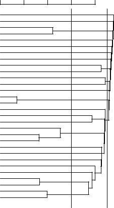
An HAC clustering is typically visualized as a dendrogram as shown in Figure 17.1. Each merge is represented by a horizontal line. The y-coordinate of the horizontal line is the similarity of the two clusters that were merged, where documents are viewed as singleton clusters. We call this similarity the combination similarity of the merged cluster. For example, the combination similarity of the cluster consisting of Lloyd’s CEO questioned and Lloyd’s chief / U.S. grilling in Figure 17.1 is ≈ 0.56. We deﬁne the combination similarity of a singleton cluster as its document’s self-similarity (which is 1.0 for cosine similarity).

By moving up from the bottom layer to the top node, a dendrogram allows us to reconstruct the history of merges that resulted in the depicted clustering. For example, we see that the two documents entitled War hero Colin Powell were merged ﬁrst in Figure 17.1 and that the last merge added Ag trade reform to a cluster consisting of the other 29 documents.

A fundamental assumption in HAC is that the merge operation is monotonic. Monotonic means that if s1, s2, . . . , sK−1 are the combination similarities of the successive merges of an HAC, then s1 ≥ s2 ≥ . . . ≥ sK−1 holds. A nonmonotonic hierarchical clustering contains at least one inversion si < si+1 and contradicts the fundamental assumption that we chose the best merge available at each step. We will see an example of an inversion in Figure 17.12.

Hierarchical clustering does not require a prespeciﬁed number of clusters. However, in some applications we want a partition of disjoint clusters just as

UP Cambridge 2009(c) edition Online

cuts possible Two .RCV1-Reuters .clusters 12 into 1.0 at and	dendrogram A 1.17 Figure
shown: are dendrogram the of	of clustering link-single a of
clusters 24 into 4.0 at	from documents 30

1.0

0.8

0.6

0.4

0.2

0.0

Ag trade reform. Back−to−school spending is up

Lloyd’s CEO questioned Lloyd’s chief / U.S. grilling Viag stays positive Chrysler / Latin America

Ohio Blue Cross Japanese prime minister / Mexico

CompuServe reports loss Sprint / Internet access service Planet Hollywood Trocadero: tripling of revenues German unions split War hero Colin Powell

War hero Colin Powell Oil prices slip

Chains may raise prices Clinton signs law Lawsuit against tobacco companies

suits against tobacco firms Indiana tobacco lawsuit Most active stocks

Mexican markets Hog prices tumble

NYSE closing averages

British FTSE index Fed holds interest rates steady

Fed to keep interest rates steady Fed keeps interest rates steady Fed keeps interest rates steady

clustering agglomerative Hierarchical 1.17

379

380	17 Hierarchical clustering

in ﬂat clustering. In those cases, the hierarchy needs to be cut at some point. A number of criteria can be used to determine the cutting point:

•Cut at a prespeciﬁed level of similarity. For example, we cut the dendrogram at 0.4 if we want clusters with a minimum combination similarity of 0.4. In Figure 17.1, cutting the diagram at y = 0.4 yields 24 clusters (grouping only documents with high similarity together) and cutting it at y = 0.1 yields 12 clusters (one large ﬁnancial news cluster and 11 smaller clusters).

•Cut the dendrogram where the gap between two successive combination similarities is largest. Such large gaps arguably indicate “natural” clusterings. Adding one more cluster decreases the quality of the clustering signiﬁcantly, so cutting before this steep decrease occurs is desirable. This strategy is analogous to looking for the knee in the K-means graph in Figure 16.8 (page 366).

•Apply Equation (16.11) (page 366):

K = arg min[RSS(K′) + λK′]

K′

where K′ refers to the cut of the hierarchy that results in K′ clusters, RSS is the residual sum of squares and λ is a penalty for each additional cluster. Instead of RSS, another measure of distortion can be used.

•As in ﬂat clustering, we can also prespecify the number of clusters K and select the cutting point that produces K clusters.

A simple, naive HAC algorithm is shown in Figure 17.2. We ﬁrst compute the N × N similarity matrix C. The algorithm then executes N − 1 steps of merging the currently most similar clusters. In each iteration, the two most similar clusters are merged and the rows and columns of the merged cluster i in C are updated.2 The clustering is stored as a list of merges in A. I indicates which clusters are still available to be merged. The function SIM(i, m, j) computes the similarity of cluster j with the merge of clusters i and m. For some HAC algorithms, SIM(i, m, j) is simply a function of C[j][i] and C[j][m], for example, the maximum of these two values for single-link.

We will now reﬁne this algorithm for the different similarity measures of single-link and complete-link clustering (Section 17.2) and group-average and centroid clustering (Sections 17.3 and 17.4). The merge criteria of these four variants of HAC are shown in Figure 17.3.

2. We assume that we use a deterministic method for breaking ties, such as always choose the merge that is the ﬁrst cluster with respect to a total ordering of the subsets of the document set

17.1 Hierarchical agglomerative clustering

381

SIMPLEHAC(d1, . . . , dN)

1	for n ← 1 to N
2	do for i ← 1 to N
3	do C[n][i] ← SIM(dn, di)
4	I[n] ← 1 (keeps track of active clusters)
5	A ← [] (assembles clustering as a sequence of merges)
6	for k ← 1 to N − 1
7	do hi, mi ← arg max{hi,mi:i6=m I[i]=1 I[m]=1} C[i][m]

8A.APPEND(hi, mi) (store merge)

9for j ← 1 to N

10do C[i][j] ← SIM(i, m, j)

11C[j][i] ← SIM(i, m, j)

12I[m] ← 0 (deactivate cluster)

13return A

Figure 17.2 A simple, but inefﬁcient HAC algorithm.

b	b
b	b
b	b
b	b

(a) single-link: maximum similarity (b) complete-link: minimum similarity

b	b
b	b
b	b
b	b

(c)centroid: average inter-similarity (d) group-average: average of all similarities

Figure 17.3 The different notions of cluster similarity used by the four HAC algorithms. An inter-similarity is a similarity between two documents from different clusters.

382	17 Hierarchical clustering

	d1	d2	d3	d4		d1	d2	d3	d4
3	×	×	×	×	3	×	×	×	×
2	d5	d6	d7	d8	2	d5	d6	d7	d8
	d5	d6	d7	d8		d5	d6	d7	d8
1	×	×	×	×	1	×	×	×	×
0					0
0	1	2	3	4	0	1	2	3	4

Figure 17.4 A single-link (left) and complete-link (right) clustering of eight documents. The ellipses correspond to successive clustering stages. Left: The single-link similarity of the two upper two-point clusters is the similarity of d2 and d3 (solid line), which is greater than the single-link similarity of the two left two-point clusters (dashed line). Right: The complete-link similarity of the two upper two-point clusters is the similarity of d1 and d4 (dashed line), which is smaller than the complete-link similarity of the two left two-point clusters (solid line).

17.2Single-link and complete-link clustering

SINGLE-LINK

CLUSTERING

COMPLETE-LINK

CLUSTERING

In single-link clustering or single-linkage clustering, the similarity of two clusters is the similarity of their most similar members (see Figure 17.3, (a))3. This single-link merge criterion is local. We pay attention solely to the area where the two clusters come closest to each other. Other, more distant parts of the cluster and the clusters’ overall structure are not taken into account.

In complete-link clustering or complete-linkage clustering, the similarity of two clusters is the similarity of their most dissimilar members (see Figure 17.3, (b)). This is equivalent to choosing the cluster pair whose merge has the smallest diameter. This complete-link merge criterion is non-local; the entire structure of the clustering can inﬂuence merge decisions. This results in a preference for compact clusters with small diameters over long, straggly clusters, but also causes sensitivity to outliers. A single document far from the center can increase diameters of candidate merge clusters dramatically and completely change the ﬁnal clustering.

Figure 17.4 depicts a single-link and a complete-link clustering of eight documents. The ﬁrst four steps, each producing a cluster consisting of a pair of two documents, are identical. Then single-link clustering joins the upper two pairs (and after that the lower two pairs) because on the maximum-

similarity deﬁnition of cluster similarity, those two clusters are closest. Complete-

3. Throughout this chapter, we equate similarity with proximity in 2D depictions of clustering.

UP Cambridge 2009(c) edition Online

clustered were	5.17 Figure
link-single with	dendrogram A
in clustering	completea of
.1.17 Figure	clusteringlink-
	documents 30 same The .

1.0	0.8	0.6	0.4	0.2	0.0

NYSE closing averages Hog prices tumble Oil prices slip Ag trade reform.

Chrysler / Latin America Japanese prime minister / Mexico Fed holds interest rates steady Fed to keep interest rates steady Fed keeps interest rates steady Fed keeps interest rates steady Mexican markets British FTSE index War hero Colin Powell War hero Colin Powell

Lloyd’s CEO questioned Lloyd’s chief / U.S. grilling

Ohio Blue Cross Lawsuit against tobacco companies suits against tobacco firms Indiana tobacco lawsuit Viag stays positive Most active stocks

CompuServe reports loss Sprint / Internet access service Planet Hollywood Trocadero: tripling of revenues

Back−to−school spending is up German unions split

Chains may raise prices Clinton signs law

clustering link-complete and link-Single 2.17

383

384	17 Hierarchical clustering

× × × × × ×

CONNECTED COMPONENT CLIQUE

Figure 17.6 Chaining in single-link clustering. The local criterion in single-link clustering can cause undesirable elongated clusters.

link clustering joins the left two pairs (and then the right two pairs) because those are the closest pairs according to the minimum-similarity deﬁnition of cluster similarity.4

Figure 17.1 is an example of a single-link clustering of a set of documents and Figure 17.5 is the complete-link clustering of the same set. When cutting the last merge in Figure 17.5, we obtain two clusters of similar size (documents 1–16, from NYSE closing averages to Lloyd’s chief / U.S. grilling, and documents 17–30, from Ohio Blue Cross to Clinton signs law). There is no cut of the dendrogram in Figure 17.1 that would give us an equally balanced clustering.

Both single-link and complete-link clustering have graph-theoretic interpretations. Deﬁne sk to be the combination similarity of the two clusters merged in step k, and G(sk) the graph that links all data points with a similarity of at least sk. Then the clusters after step k in single-link clustering are the connected components of G(sk) and the clusters after step k in complete-link clustering are maximal cliques of G(sk). A connected component is a maximal set of connected points such that there is a path connecting each pair. A clique is a set of points that are completely linked with each other.

These graph-theoretic interpretations motivate the terms single-link and complete-link clustering. Single-link clusters at step k are maximal sets of points that are linked via at least one link (a single link) of similarity s ≥ sk; complete-link clusters at step k are maximal sets of points that are completely linked with each other via links of similarity s ≥ sk.

Single-link and complete-link clustering reduce the assessment of cluster quality to a single similarity between a pair of documents: the two most similar documents in single-link clustering and the two most dissimilar documents in complete-link clustering. A measurement based on one pair cannot fully reﬂect the distribution of documents in a cluster. It is therefore not surprising that both algorithms often produce undesirable clusters. Single-link clustering can produce straggling clusters as shown in Figure 17.6. Since the merge criterion is strictly local, a chain of points can be extended for long

4. If you are bothered by the possibility of ties, assume that d1 has coordinates (1 + ǫ, 3 − ǫ) and that all other points have integer coordinates.

<<< < Предыдущая 80 81 82 83 84 85 86 87 88 89 90 9192 / 12192 93 94 95 96 97 98 99 100 101 102 103 104 > Следующая >>>

Соседние файлы в предмете [НЕСОРТИРОВАННОЕ]

#
02.06.2015108.48 Кб4Amirbekov.pdf
#
02.06.2015557.57 Кб60An Intensive Course of English Writing.doc
#
02.06.20151.08 Mб5Anderson_Rio_Gangster.pdf
#
18.12.2018721.41 Кб4antigtu.ru-shpora_po_teorii_veroyatnosti_disper....doc
#
02.06.2015108.54 Кб12Antipeva_chto_to_25_04_14.doc
#
26.03.20166.9 Mб419An_Introduction_to_Information_Retrieval.pdf
#
02.06.2015833.24 Кб2APK_(01.01.2012).rtf
#
02.06.2015846.45 Кб4APK_(24.09.2012).rtf
#
26.03.2016355.36 Кб13Arabic_London.docx
#
07.09.201923.88 Кб4Armenia.docx
#
02.06.2015141.86 Кб3article1381160542_Unegbu and Tasie.pdf

	d1	d2	d3	d4		d1	d2	d3	d4
3	×	×	×	×	3	×	×	×	×
2	d5	d6	d7	d8	2	d5	d6	d7	d8
	d5	d6	d7	d8		d5	d6	d7	d8
1	×	×	×	×	1	×	×	×	×
0					0
0	1	2	3	4	0	1	2	3	4

	d1	d2	d3	d4		d1	d2	d3	d4
3	×	×	×	×	3	×	×	×	×
2	d5	d6	d7	d8	2	d5	d6	d7	d8
	d5	d6	d7	d8		d5	d6	d7	d8
1	×	×	×	×	1	×	×	×	×
0					0
0	1	2	3	4	0	1	2	3	4

	d1	d2	d3	d4		d1	d2	d3	d4
3	×	×	×	×	3	×	×	×	×
2	d5	d6	d7	d8	2	d5	d6	d7	d8
	d5	d6	d7	d8		d5	d6	d7	d8
1	×	×	×	×	1	×	×	×	×
0					0
0	1	2	3	4	0	1	2	3	4