~xj

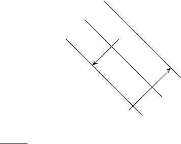
Figure 15.5 Large margin classification with slack variables.

15.2Extensions to the SVM model

15.2.1Soft margin classification

For the very high dimensional problems common in text classification, sometimes the data are linearly separable. But in the general case they are not, and even if they are, we might prefer a solution that better separates the bulk of the data while ignoring a few weird noise documents.

If the training set D is not linearly separable, the standard approach is to allow the fat decision margin to make a few mistakes (some points – outliers or noisy examples – are inside or on the wrong side of the margin). We then pay a cost for each misclassified example, which depends on how far it is from meeting the margin requirement given in Equation (15.5). To imple-

SLACK VARIABLES ment this, we introduce slack variables ξi. A non-zero value for ξi allows ~xi to not meet the margin requirement at a cost proportional to the value of ξi. See Figure 15.5.

The formulation of the SVM optimization problem with slack variables is:

(15.10) Find w~ , b, and ξi ≥ 0 such that:

•12 w~ Tw~ + C ∑i ξi is minimized

•and for all {(~xi, yi)}, yi(w~ T~xi + b) ≥ 1 − ξi

Online edition (c) 2009 Cambridge UP

The optimization problem is then trading off how fat it can make the margin versus how many points have to be moved around to allow this margin. The margin can be less than 1 for a point ~xi by setting ξi > 0, but then one pays a penalty of Cξi in the minimization for having done that. The sum of the ξi gives an upper bound on the number of training errors. Soft-margin SVMs minimize training error traded off against margin. The parameter C

REGULARIZATION is a regularization term, which provides a way to control overfitting: as C becomes large, it is unattractive to not respect the data at the cost of reducing the geometric margin; when it is small, it is easy to account for some data points with the use of slack variables and to have a fat margin placed so it models the bulk of the data.

The dual problem for soft margin classification becomes:

(15.11) Find α1, . . . αN such that ∑ αi − 12 ∑i ∑j αiαjyiyj~xiT~xj is maximized, and

•∑i αiyi = 0

•0 ≤ αi ≤ C for all 1 ≤ i ≤ N

Neither the slack variables ξi nor Lagrange multipliers for them appear in the dual problem. All we are left with is the constant C bounding the possible size of the Lagrange multipliers for the support vector data points. As before, the ~xi with non-zero αi will be the support vectors. The solution of the dual problem is of the form:

(15.12) w~ = ∑ αyi~xi

b = yk(1 − ξk) − w~ T~xk for k = arg maxk αk

Again w~ is not needed explicitly for classification, which can be done in terms of dot products with data points, as in Equation (15.9).

Typically, the support vectors will be a small proportion of the training data. However, if the problem is non-separable or with small margin, then every data point which is misclassified or within the margin will have a nonzero αi. If this set of points becomes large, then, for the nonlinear case which we turn to in Section 15.2.3, this can be a major slowdown for using SVMs at test time.

The complexity of training and testing with linear SVMs is shown in Table 15.1.3 The time for training an SVM is dominated by the time for solving the underlying QP, and so the theoretical and empirical complexity varies depending on the method used to solve it. The standard result for solving QPs is that it takes time cubic in the size of the data set (Kozlov et al. 1979). All the recent work on SVM training has worked to reduce that complexity, often by

3. We write Θ(|D|Lave) for Θ(T) (page 262) and assume that the length of test documents is bounded as we did on page 262.

Online edition (c) 2009 Cambridge UP

Table 15.1 Training and testing complexity of various classifiers including SVMs. Training is the time the learning method takes to learn a classifier over D, while testing is the time it takes a classifier to classify one document. For SVMs, multiclass classification is assumed to be done by a set of |C| one-versus-rest classifiers. Lave is the average number of tokens per document, while Mave is the average vocabulary (number of non-zero features) of a document. La and Ma are the numbers of tokens and types, respectively, in the test document.

being satisfied with approximate solutions. Standardly, empirical complexity is about O(|D|1.7) (Joachims 2006a). Nevertheless, the super-linear training time of traditional SVM algorithms makes them difficult or impossible to use on very large training data sets. Alternative traditional SVM solution algorithms which are linear in the number of training examples scale badly with a large number of features, which is another standard attribute of text problems. However, a new training algorithm based on cutting plane techniques gives a promising answer to this issue by having running time linear in the number of training examples and the number of non-zero features in examples (Joachims 2006a). Nevertheless, the actual speed of doing quadratic optimization remains much slower than simply counting terms as is done in a Naive Bayes model. Extending SVM algorithms to nonlinear SVMs, as in the next section, standardly increases training complexity by a factor of |D| (since dot products between examples need to be calculated), making them impractical. In practice it can often be cheaper to materialize

Online edition (c) 2009 Cambridge UP

the higher-order features and to train a linear SVM.4

15.2.2Multiclass SVMs

SVMs are inherently two-class classifiers. The traditional way to do multiclass classification with SVMs is to use one of the methods discussed in Section 14.5 (page 306). In particular, the most common technique in practice has been to build |C| one-versus-rest classifiers (commonly referred to as “one-versus-all” or OVA classification), and to choose the class which classifies the test datum with greatest margin. Another strategy is to build a set of one-versus-one classifiers, and to choose the class that is selected by the most classifiers. While this involves building |C|(|C| − 1)/2 classifiers, the time for training classifiers may actually decrease, since the training data set for each classifier is much smaller.

However, these are not very elegant approaches to solving multiclass problems. A better alternative is provided by the construction of multiclass SVMs, where we build a two-class classifier over a feature vector Φ(~x, y) derived

from the pair consisting of the input features and the class of the datum. At

test time, the classifier chooses the class y = arg maxy′ w~ TΦ(~x, y′). The margin during training is the gap between this value for the correct class and for the nearest other class, and so the quadratic program formulation will

require that i y 6= yi w~ TΦ(~xi, yi) − w~ TΦ(~xi, y) ≥ 1 − ξi. This general method can be extended to give a multiclass formulation of various kinds of linear classifiers. It is also a simple instance of a generalization of classifica-

tion where the classes are not just a set of independent, categorical labels, but may be arbitrary structured objects with relationships defined between them.

STRUCTURAL SVMS In the SVM world, such work comes under the label of structural SVMs. We mention them again in Section 15.4.2.

15.2.3Nonlinear SVMs

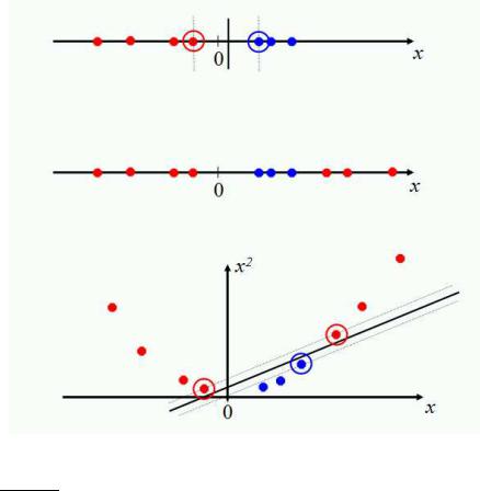
With what we have presented so far, data sets that are linearly separable (perhaps with a few exceptions or some noise) are well-handled. But what are we going to do if the data set just doesn’t allow classification by a linear classifier? Let us look at a one-dimensional case. The top data set in Figure 15.6 is straightforwardly classified by a linear classifier but the middle data set is not. We instead need to be able to pick out an interval. One way to solve this problem is to map the data on to a higher dimensional space and then to use a linear classifier in the higher dimensional space. For example, the bottom part of the figure shows that a linear separator can easily classify the data

4. Materializing the features refers to directly calculating higher order and interaction terms and then putting them into a linear model.

Online edition (c) 2009 Cambridge UP

Figure 15.6 Projecting data that is not linearly separable into a higher dimensional space can make it linearly separable.

if we use a quadratic function to map the data into two dimensions (a polar coordinates projection would be another possibility). The general idea is to map the original feature space to some higher-dimensional feature space where the training set is separable. Of course, we would want to do so in ways that preserve relevant dimensions of relatedness between data points, so that the resultant classifier should still generalize well.

SVMs, and also a number of other linear classifiers, provide an easy and efficient way of doing this mapping to a higher dimensional space, which is KERNEL TRICK referred to as “the kernel trick”. It’s not really a trick: it just exploits the math that we have seen. The SVM linear classifier relies on a dot product between data point vectors. Let K(~xi,~xj) = ~xiT~xj. Then the classifier we have seen so

Online edition (c) 2009 Cambridge UP

Online edition (c) 2009 Cambridge UP