Добавил:

Upload Опубликованный материал нарушает ваши авторские права? Сообщите нам.

Вуз:

Национальный исследовательский университет «Высшая школа экономики»

Предмет:

[НЕСОРТИРОВАННОЕ]

Файл:

david_Introduction_to_behavioral_economics.pdf

Скачиваний:

Добавлен:

26.03.2016

Размер:

12.18 Mб

Скачать

☆

<<< < Предыдущая 42 43 44 45 46 47 48 49 50 51 52 5354 / 7654 55 56 57 58 59 60 61 62 63 64 65 66 > Следующая >>>


	318		NAÏVE PROCRASTINATION

slope = δ –j–1 K slope = δ –j K

u(c)

slope = δ –j–n K

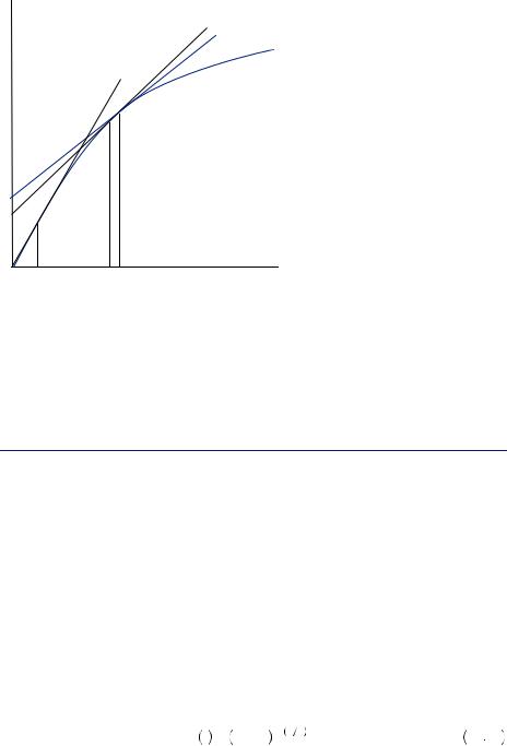
FIGURE 12.3
Consumption	cj + n	cj +1 cj	c
Smoothing

Alternatively, in the SNAP data, we observe a sharp decline in food consumption in the last week. This signals yet again that the behavior is contradicting the standard economic model of choice. The rational model suggests that recipients will have the foresight to conserve their money to consume similar amounts every day rather than consume a lot up front and then run out of food and money in the last week of the month. A time-consistent model of decision making would not predict this behavior, nor can it be reconciled.

Naïve Hyperbolic Discounting

Robert H. Strotz ﬁrst proposed a model of time-inconsistent preferences due to discounting that varies by the time horizon. Generally, he examined cases in which discount factors in the near term are relatively small, indicating that consumption now is much more valuable than in the near future. However, discount factors in the distant future are much closer to 1. His proposed model was used primarily as a method to explore the potential generalizations of the common exponential discounting model that might permit time-inconsistent preferences. Since his proposal, many have found empirical support for the notion of timeinconsistent preferences; George W. Ainsley proposed a model that, with some later modiﬁcations, is commonly called hyperbolic discounting. Hyperbolic discounting replaces the common exponential discount, δt, with the hyperbolic discount factor

h t = 1 + αt − β α ,

12 19

where β, α > 0 are parameters and t is the amount of time that will have passed by the instance of consumption. Thus, the consumer maximizes


Naïve Hyperbolic Discounting		319

Discount factor

Time discounting

0.9

0.8

0.7

0.6

0.5

0.4

0.3

0.2

0.1

0 0	5	10	15	20	25
			Time

FIGURE 12.4

Hyperbolic (Squares) and Quasi-Hyperbolic

(Triangles) Time Discounting

max c1, c2, U c1, c2,	=	1 + αi − β α	u ci .	12 20
		T

i = 1

Ainsley has found this form to be consistent with the behavior of animals in behavioral experiments introducing intertemporal choice, as well as with human behavior in similar experiments. Figure 12.4 displays the hyperbolic discount factor as well as the exponential discount factor for up to 25 time periods. The squares mark the hyperbolic discount factor and the circles mark the exponential discount factor. The hyperbolic discount factor declines very quickly over the ﬁrst few time periods compared to the exponential discount function. Thus, a consumer behaving according to hyperbolic discounting will value near-term future consumption much less than someone who discounts according to exponential discounting. Alternatively, the hyperbolic discount function declines very slowly over the latter periods relative to the exponential discount function. Thus, a consumer who displays hyperbolic time discounting is much more willing to delay consumption in the distant future than in the near future. Values of the hyperbolic discount function for various parameter values and selected periods are displayed in Table 12.1. Note that the discount factor is increasing in α and decreasing in β and t.

Consider two questions posed by Richard Thaler. The ﬁrst question is, “Would you rather have one apple today or two apples tomorrow?” Many people, when posed this question, consider that it is not worth it to wait a whole day just to obtain an additional apple. Thus, they elect to have the apple today. Let u1 be the instantaneous utility obtained from eating one apple, u2 be the instantaneous utility obtained from eating two apples, and δ the daily discount factor applied to decisions for consumption today versus tomorrow. Then choosing the apple today instead of two tomorrow implies u1 > δu2. Now consider the second question: “Would you rather have one apple one year from now, or two apples one year and one day from now?” Many respond to this


320		NAÏVE PROCRASTINATION
		Table 12.1 Values of the Hyperbolic Discount Function
		for Various Parameters

		α =	β =	t =1	t = 2				t =5		t =20	t =100	t =200

	0.10		0.10	0.91	0.83				0.67		0.33	0.09	0.05
	0.20		0.10	0.91	0.85				0.71		0.45	0.22	0.16
	0.50		0.10	0.92	0.87				0.78		0.62	0.46	0.40
	1.00		0.10	0.93	0.90				0.84		0.74	0.63	0.59
	2.00		0.10	0.95	0.92				0.89		0.83	0.77	0.74
	0.10		0.20	0.83	0.69				0.44		0.11	0.01	0.00
	0.20		0.20	0.83	0.71				0.50		0.20	0.05	0.02
	0.50		0.20	0.85	0.76				0.61		0.38	0.21	0.16
	1.00		0.20	0.87	0.80				0.70		0.54	0.40	0.35
	2.00		0.20	0.90	0.85				0.79		0.69	0.59	0.55
	0.10		0.50	0.62	0.40				0.13		0.00	0.00	0.00
	0.20		0.50	0.63	0.43				0.18		0.02	0.00	0.00
	0.50		0.50	0.67	0.50				0.29		0.09	0.02	0.01
	1.00		0.50	0.71	0.58				0.41		0.22	0.10	0.07
	2.00		0.50	0.76	0.67				0.55		0.40	0.27	0.22

		question by thinking one year and a day is not much different from waiting one year, and
		this small wait will result in twice the number of apples. Thus the majority select to wait
		the extra day. This is a clear violation of the stationarity property described earlier in
		this chapter.
		Let ψ be the daily discount factor for decisions regarding consumption one year from
		now	and γ the	discount	applied for				waiting		one year. This	then	implies that
		γu 1	< γψu 2 . Choosing one apple today and two apples a year and a day from now
	can only be reconciled if δ < ψ—if the daily percentage discount decreases over time.
	The hyperbolic discount rate can accommodate this difference. For example, the
	hyperbolic discount rate for period 0								(today),		and period 1(tomorrow) would be
		1 − β α = 1 and		1 + α − β α . Thus δ = 1 + α − β α < 1. If α is large enough, δ is
		much smaller than 1. Alternatively, the discount applied to one year out and one year
		and one day are		1 + α365	− β α	and			1 + α366		− β α , respectively. Thus the daily
		discount one year out is
					ψ =	1 +			α366	− αβ	1.		12 21
						1 +			α366

							1 + α365
		This is a potential solution to the apple conundrum.
		In general, the discount factor applied from one period to the next has the form
					ψ t =			1 + α t + 1			− αβ
								1 + α t + 1			,		12 22
											,		12 22
									1 + αt


Naïve Hyperbolic Discounting		321

which converges to ψt = 1 as t increases toward inﬁnity. Thus, in the long run the period-by-period discount rate always goes to 1. Alternatively, the rate can be quite small for smaller values of t, particularly if α is large. If instead α is small, elementary calculus tells us that the value of the discount factor converges to

limα 0ψ t = e − β,

12 23

which is a constant. Thus, when α is very small, the hyperbolic discount function behaves much like exponential discounting, with δ = e − β.

Let us revisit the behavior observed by food stamp (or SNAP) participants. If they display a sharply higher level of consumption in the ﬁrst week of the month than in the last, it may be due to hyperbolic time discounting. If a SNAP recipient is a hyperbolic discounter, then on the ﬁrst day of the month, she will solve

max x, c0, c30 v x +	30	+ αt	− β α u ct
max x, c0, c30 v x +	1	+ αt	− β α u ct	12 24
	t = 0

subject to the constraints equations 12.16 and 12.17. Now instead of equation 12.18, the consumption for any two periods j and k must conform to

1 + αj − αβ

u′ cj = 1 + αk − αβ

u′ ck ,

12 25

where, as before, u′c is the marginal instantaneous utility function evaluated at c, and let j < k. Equation 12.25 implies that the discount applied to the utility of consumption between any two periods j and k will be

ψ j, k =	1 + αk	−	αβ
			.	12 26
	1 + αj

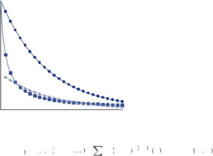
Consider the case if we hold j constant and adjust k. Because of the hyperbolic shape of the function, in many cases ψj, k is substantially lower than one when j and k are relatively close together. Thus, as pictured in Figure 12.5, it may be that planned consumption changes by a relatively large and abrupt amount from one period to the next. In other words, consumption might not be so smooth in the near term. The recipient might convince herself that consumption now is extremely important relative to tomorrow but that it is not nearly so important to consume tomorrow rather than the next day. 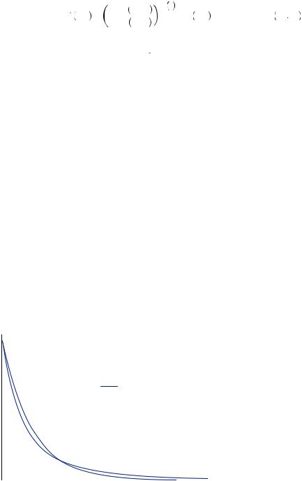Thus, because ψj, j + 1 converges to 1 as j gets large, planned consumption in the distant future will be smooth, though planned consumption in the near term is not. Thus a SNAP recipient who behaves according to hyperbolic discounting when receiving her beneﬁts will plan to consume a lot today (or maybe in the ﬁrst week) but then hope to smooth out her consumption over the rest of the month. Figure 12.6 offers another view of this behavior, where discounting between periods 1 and 2 is relatively steep, resulting in very different discounted marginal utility curves. Alternatively, discounting between periods 2 and 3 is very mild, resulting in nearly identical discounted marginal utility curves between periods 2 and 3 when planning from the point of view of period 1.


	322		NAÏVE PROCRASTINATION

FIGURE 12.5

Hyperbolic Discounting Increases Current Relative to Future Consumption

FIGURE 12.6

Consumption Nonsmoothing under Hyperbolic Discounting

slope = h( j+1)–1 K slope = h( j)–1 K

u(c)

slope = h( j+n)–1 K

cj + n	cj +1	cj			c
utility	u'(c1)		ψ (1,2)u'(c2)		ψ (1,3)u'(c3)
Discounted marginal	u'(c1)		ψ (1,2)u'(c2)		ψ (1,3)u'(c3)
Discounted marginal
c1	c1	c2	c2	c3	c3

But then the rest of the month happens. Unfortunately with time-inconsistent preferences, the recipient does not live by her plan. Instead, when she arrives in the second period, she solves

max c1, c30	30	+ α t − 1	− β α u ct
max c1, c30	1	+ α t − 1	− β α u ct	12 27
	t = 1

subject to new constraints that reﬂect the consumption of the ﬁrst day. The new time index in the discount factor reﬂects that now the recipient is making her plans in period 1 rather than period 0. Thus, now consumption in period 1 enjoys a favored status relative to period 2 and all future periods. The new solution must satisfy

1 + α j − 1 − αβ

u′ cj = 1 + α k − 1 − αβ

u′ ck .

12 28

So, where before the difference in the slope of the utility function for consumption in periods j and k could be represented by equation 12.26, now it is represented by


			Naïve Hyperbolic Discounting		323
ψ j, k =	1 + α k − 1	− αβ	< ψ j, k .	12 29
ψ j, k =		− αβ	< ψ j, k .	12 29
	1 + α j − 1

Previously, recipients had anticipated applying a discount of ψ1, 2 between the ﬁrst and second periods. Now instead, they apply ψ1, 2 = ψ0, 1. Thus, despite the plans made previously, recipients now feel that they need to consume more now relative to the future. They thus consume more in period 1 than they had planned, leaving less for the future when they anticipated smoothing their consumption. In the following period, they again decide to consume more than they had planned to in either of the previous periods, again putting off consumption smoothing until a later date. Recipients continue to put off smoothing until they reach a point where they no longer have enough food to last the rest of the month, and their consumption is forced to drop off signiﬁcantly.

Figure 12.7 displays the planned consumption on the ﬁrst day of the month for the SNAP problem given a utility of food consumption function, uc = c0.7 and a hyperbolic discounting function with α = 0.1, β = 1. The planned consumption is much higher at the beginning of the month than at the end, but it allows some steady but low level of consumption from about day 20 of the monthly cycle onward. Alternatively, the actual level of consumption is obtained by solving the optimization again each period with a new discount function as given in equation 12.28. In this case, recipients decide once they are in the second period that they should consume more than they had planned. They continue to revise their consumption upward until the ninth period. After that, their budget does not allow them to continue to consume more than they had planned. Feast then turns to famine. At that point, they must begin consuming less and less. Consumption in the last 10 days is less than 1/10 of planned consumption and is nearly zero.

Hyperbolic discounting is a relatively simple way to represent the type of presentbiased preferences, or an extreme discounting of the future, that seems the only explanation for such procrastination behavior. The model suggests that people plan to

Consumption

Planned versus actual consumption

15					Planned consumption
					Planned consumption
10					Actual consumption
					Actual consumption


5
0								FIGURE 12.7

	0	5	10	15	20	25	30 The SNAP Problem with Hyperbolic Dis-
				Time				counting

<<< < Предыдущая 42 43 44 45 46 47 48 49 50 51 52 5354 / 7654 55 56 57 58 59 60 61 62 63 64 65 66 > Следующая >>>

Соседние файлы в предмете [НЕСОРТИРОВАННОЕ]

#
05.12.2018329.73 Кб2CS_SUFF_2011_1.doc
#
08.12.2018413.18 Кб3CS_SUFF_2011_1.doc
#
26.03.201685.5 Кб13cеминар 5 _Эластичность спроса.doc
#
02.06.2015210.43 Кб384Cловарь терминов МЧП.doc
#
02.06.2015200.7 Кб133Cхемы по МЧП.doc
#
26.03.201612.18 Mб50david_Introduction_to_behavioral_economics.pdf
#
26.03.2016230.91 Кб6default.doc
#
11.11.201930.35 Кб1Definitions.docx
#
02.06.201582.36 Кб11Democracy_and_Economic_Development.pdf
#
26.03.201633.34 Mб27Diagrammy_v_Excel_Dzhon_Uokenbakh_2003.pdf
#
26.03.2016194.23 Кб7Dictatorship_and_Democracy_19181939.pdf