

|
|
|
|
An Evolutionary Explanation for Loss Aversion |
|
81 |
|
x2
r2
r1 |
FIGURE 4.4 |
x1 Indifference Curves with Constant Loss Aversion |
λi > 1, exaggerating the impact of losses, and creating a kink in the value function at the reference point in each dimension. We refer to the reference structure as displaying
constant additive loss aversion if we can write the utility function as vr x = n |
Ri xi . |
i = |
1 |
This is consistent with assuming that someone displays preferences that are loss averse over each good and that goods are not substitutes or complements.
If the reference structure displays constant loss aversion, the indifference curves take on a relatively intuitive shape as displayed in Figure 4.4. In each quadrant, the indifference curves are parallel. However, each indifference curve is kinked as it crosses the reference line in any dimension. Indifference curves become steeper in the northwest quadrant because more of good 2 is needed to compensate for the loss of good 1. Indifference curves become flatter in the southeast quadrant because it requires more of good 1 to compensate for losses of good 2. Indifference curves in the northeast and southwest quadrants have an intermediate slope because here both goods have the same loss or gain status. A derivation of the indifference curves under constant loss aversion is presented in the Advanced Concept box found at the end of this chapter for the interested reader. Indifference curves with flat portions create a possibility that the point of tangency with a budget constraint is not particularly sensitive to price changes. In other words, as the slope of the budget constraint changes, over a relatively wide range of prices the same kink point will likely be the optimum, leading to a sort of status quo bias in consumption bundles.
An Evolutionary Explanation for Loss Aversion
Although it seems intuitive why people would want to maximize their utility, it is a little more difficult to understand why their utility might be reference dependent. It seems that one would be better off on average if one behaved according to standard utility maximization, and thus one potentially has a greater chance to survive and procreate, passing

|
|
|
|
|
82 |
|
STATUS QUO BIAS AND DEFAULT OPTIONS |
one’s genes down to future generations. Instead, our bodies appear to have evolved and adapted to perceive changes and ignore the status quo. You might experience this when someone turns on the light in an otherwise dark room. As soon as the light goes on, it can be painful and annoying. After a brief adjustment period, the eyes adjust for the added light and the light becomes pleasant, or at least not of any note. We react to temperature, pain, or background noise in much the same way.
A good illustration is given in one of the exhibits in San Francisco’s Exploratorium. When you first approach this exhibit, a small plastic card with a light shining on it appears. When you inspect the card, it appears to be white. Then, a second card appears directly next to the first, only it is much brighter. Now it becomes clear that the first card was not white at all, but slightly gray, and the second card appears white. This process of cards appearing continues until, at last, you realize the first card was actually pitch black. Only because it appeared with a light shining on it and with no other cards to use as a reference did it appear to be white.
We are hard wired to use references and changes in our decisions. This may be useful on an evolutionary basis. Imagine the world if you experienced every sensation just as keenly at every instant whether changes were occurring or not. When you were bitten by an unseen snake or burned by some unexpectedly hot item, you might not react quickly enough because it would not draw your attention significantly. If you tend not to notice anything until a change occurs, the snake or burn draws immediate attention, providing you time to react before serious damage is done.
Evidence of loss aversion as a hard-wired trait comes from the work of Keith Chen, Venkat Lakshminarayanan, and Laurie Santos. They studied a colony of capuchin monkeys. By introducing a currency among the monkeys, they could observe trades and run economic experiments. In their study they found that monkeys tend to display loss aversion under many of the same circumstances in which it is found in human behavior. Because these monkeys lack the type of social communication found among humans, the researchers conclude that the behavior is inherited rather than learned. Thus, loss aversion may be an adaptation driven by evolutionary pressures rather than a skill learned from social interactions or from training as a child.
EXAMPLE 4.6 The Endowment Effect
Suppose you have just purchased a new car. You ordered the car online choosing all of the options you wanted and then picked the vehicle up from the dealer several days later. After driving the car home, you park it in your garage and spend a few minutes admiring the new vehicle. Upon entering your home, you discover a phone message from the dealer. Apparently someone else had ordered a car that was identical in every respect, except the sound system was not quite as powerful as you had wanted. The dealership accidentally sent you home with the wrong car. They inform you that you can drive back and exchange the vehicle for the one you ordered. You consider exchanging for a moment, but then decide to let the other person have the car you ordered. Driving the other car would not quite be the same as the car you have already come to know. Several weeks later you upgrade the sound system as you had originally desired.

|
|
|
|
Rational Choice and Getting and Giving Up Goods |
|
83 |
|
Rational Choice and Getting and Giving Up Goods
The rational model of choice supposes that the change in utility upon receiving a good is identical to the amount that would be lost if the good is taken away. Consider the case where someone who is consuming none of good 1 and some amount of good 2, given by x2. Her utility can be written as u 0, x2
0, x2 . If she is given an amount of good 1, x1, her utility increases by the amount u
 x1, x2
 − u
− u 0, x2
0, x2 . If the amount of good 1 is subsequently taken away, she loses utility u
 x1, x2
 − u
− u 0, x2
0, x2 , resulting in the original level of utility, u
 0, x2
0, x2 .
.
Consider also the problem of determining the maximum amount one is willing to pay to acquire a good. Consider someone who currently only has good 2 available to her. She
thus solves |
|
max u 0, x2 , |
4 2 |
x2 |
|
subject to the budget constraint |
|
p2x2 ≤ w, |
4 3 |
where w is wealth and p2 represents the price of good 2. If the utility function is strictly increasing in the consumption of good 2 (i.e., more of good 2 is always better), then she solves the decision problem by consuming x2* = w p2 and obtaining utility u
 0, x2*
 . Now consider this person is offered one unit of good 1. She would not be willing to buy if the purchase reduced her overall utility level. Further, if she could purchase the item and receive a greater level of utility, she could clearly pay more and still be better off. Thus, to solve for the maximum amount the decision maker is willing to pay, we must find the price for the unit of good 1 that keeps the person on the same indifference curve. Given that she purchases the unit of good 1 at a price p1, the remaining wealth is given by w − p1, which must be spent on good 2. This results in a new optimal amount of good 2 given by x2* =
  w − p1
 p2 = x2* − p1
 p2. Thus, the maximum willingness to pay (WTP) for x1 can be written as pWTP1 such that
u 1, x2* − p1WTP p2 = u 0, x2* . |
4 4 |
Now instead, let us find the minimum amount one would be willing to accept to part with the same good. Consider that someone was originally endowed with one unit of good 1, and we wished to determine how much she would be willing to sell the item for. In this case, her original consumption can be described by
max u 1, x2 , |
4 5 |
x2 |
|
subject to the budget constraint |
|
p2x2 ≤ w. |
4 6 |
|
|
|
|
|
84 |
|
STATUS QUO BIAS AND DEFAULT OPTIONS |
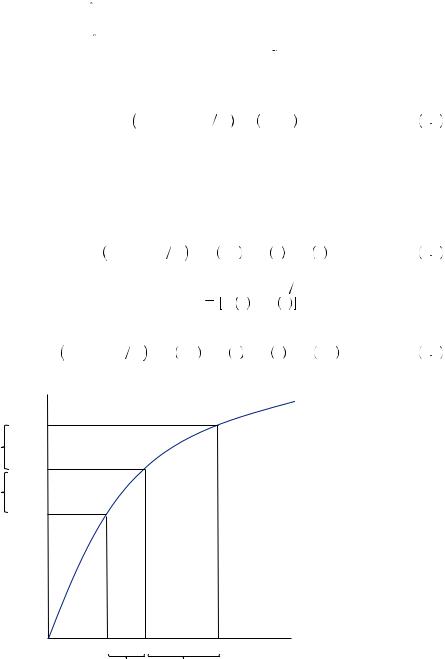
FIGURE 4.5 Disparity between Willingness to Pay (WTP) and Willingness to Accept (WTA)
This problem is solved by x2* = w p2 and results in a utility of u
 1, x2*
 . Because x2* is clearly greater than x2*, it is clear that the level of utility obtained when the person is endowed with good 1 is greater than when the person is charged the maximum willingness to pay, u
 1, x2*
 . If the person sold the unit of good 1 for p1, her budget constraint is then given by w + p1. Thus, she would choose x2* =
  w + p1
 p2 = x2* + p1
 p2. The minimum amount she is willing to take in place of the unit of good 1, or the willingness to accept (WTA), can now be written as pWTA1 such that
u 0, x2* + p1WTA p2 = u 1, x2* . |
4 7 |
It is noteworthy that equation 4.7 is not equivalent to equation 4.4 and that rational decision makers in general display a minimum WTA, pWTA1 , that is larger than their maximum WTP, pWTP1 .
To see this, consider the special case of additive utility, u x1, x2
 = u1
= u1 x1
x1 + u2
+ u2 x2
x2 . In this case, equation 4.4 implies
u2 x2* − p1WTP p2 = u2 x2* + u1 0 − u1 1 , |
4 8 |
||||
meaning that if the person had x2* of good 2, and lost p1WTP |
p2 of it, it would reduce their |
||||
utility from good 2 by the quantity |
u1 |
u1 1 |
− u1 0 |
, as pictured in Figure 4.5. |
|
Equation 4.7 implies |
|
|
|
|
|
u2 x2* + p1WTA p2 = u2 |
x2* |
+ u1 1 |
− u1 0 |
= u2 x2* + u1. |
4 9 |
u2
2 (~2*) u x
∆u1
u2 (x2*)
∆u1
u2 (xˆ2*)
xˆ2* |
x2* |
~ |
x2 |
x2* |
|||
p1WTP / p2 |
p1WTA/ p2 |
|
|