


|
|
|
|
Risk Aversion, Risk Loving, and Loss Aversion |
|
253 |
|
0.8 probability of receiving $4,000, or an overall probability of 0.25 × 0.8 = 0.2 to receive $4,000 and 0.8 of receiving nothing. Alternatively, if we choose Gamble F, we have a 0.25 chance of receiving $3,000, and a 0.75 of receiving $0. Thus we could rewrite this compound gamble as
Gamble E’: |
Gamble F’: |
$4,000 with probability 0.2 |
$3,000 with probability 0.25 |
$0 with probability 0.8 |
$0 with probability 0.75 |
|
|
Interestingly, when phrased this way, 65 percent of participants choose Gamble E over F . In this case, preferences seem to depend heavily upon how transparent the description of the gamble is. People apparently do not simplify compound lotteries the way expected utility would assume. Additionally, some participants were asked how they would choose between
Gamble E’’: |
Gamble F’’: |
$4,000 with probability 0.8 |
$3,000 with certainty |
$0 with probability 0.2 |
|
|
|
This gamble is identical to the second stage of the previous problem in isolation (gambles E and F). In this case, 80 percent of participants chose Gamble F , very similar to the 78 percent in the original problem. It appears that decision makers ignore the first stages of such a compound lottery and focus only on the latter stages. In general, we might expect participants to eliminate common components of gambles in making decisions, such as the first-stage lottery in this example.
Risk Aversion, Risk Loving, and Loss Aversion
Recall from Chapter 6 that under the theory of expected utility maximization, risk aversion is represented by a concave utility function. As the payoff for the gamble increases, the utility of the marginal dollar (the slope of the utility function) declines. This leads participants to receive less expected utility from the gamble than they would from receiving a one-time payment equal to the expected value of the gamble. Figure 10.1 displays such a utility function when the participant faces a 0.5 probability of receiving x2 dollars and a 0.5 probability of receiving x1 dollars. Thus the expected value of the gambles is given by E x
x = 0.5
= 0.5 x1 + x2
 , the point on the horizontal axis exactly halfway between x1 and x2. Alternatively, the expected utility of the gamble is given by E
 u
u x
x = 0.5
= 0.5 u
u x1
x1 + u
+ u x2
x2 , which is the point on the vertical axis that is exactly halfway between u
 x1
x1 and u
and u x2
x2 . This point will always be less than U
 0.5
0.5 x1 + x2
 when the utility function is concave. The participant would be indifferent between taking xCE < E
 x
x and taking the gamble. Thus, concavity of the utility function is associated with risk-averse behavior.

|
|
|
|
|
254 |
|
PROSPECT THEORY AND DECISION UNDER RISK OR UNCERTAINTY |
u(x) u(x2)
u(E(x))
E(u(x))
u(x1)
FIGURE 10.1 |
|
|
|
|
Risk Aversion and |
|
|
|
|
Concavity |
x1 |
xCE E(x) |
x2 |
x |
u(x) u(x2)
|
E(u(x)) |
|
|
|
|
u(E(x)) |
|
|
|
FIGURE 10.2 |
u(x1) |
|
|
|
Risk Loving and |
x1 |
|
x2 |
x |
Convexity |
E(x) xCE |
The opposite is true when the decision maker has a convex utility of wealth function. In this case, displayed in Figure 10.2, the expected utility of the gamble E u
u x
x = 0.5
= 0.5 u
u x1
x1 + u
+ u x2
x2 is always greater than U
 0.5
0.5 x1 + x2
 . Because the utility function is convex, the point on the utility function that corresponds to the point on the vertical axis that is halfway between u
 x1
x1 and u
and u x2
x2 is always to the right of the expected value of the gamble. Decision makers would be indifferent between taking xCE > E
 x
x and taking the gamble. With a convex utility function, decision makers are made better off by taking the gamble than by taking an amount of money equal to the expected value of the
|
|
|
|
Risk Aversion, Risk Loving, and Loss Aversion |
|
255 |
|
gamble. In other words, they are risk loving. Thus, convexity of the utility function is associated with risk-loving behavior.
In previous chapters, “loss aversion” has been used to describe behavior in the context of consumer choices. For example, people tend to display the sunk cost fallacy when they classify sunk costs as a loss and future benefits from continuing an activity as a gain associated with that loss (see the section on “Theory and Reactions to Sunk Cost” in Chapter 2). Kahneman and Tversky proposed prospect theory based on the notion that people classify each event as either a gain or a loss and then evaluate gains and losses using separate utility functions. Gains are evaluated via a utility function over gains, which we have called ug x
x , that is concave. Thus people display diminishing marginal utility over gains. In the context of gambles and lotteries, the argument of the utility function is wealth, or the money outcome of the gamble. Thus, the utility function over gains displays diminishing marginal utility of wealth, which is associated with riskaverse behavior. Losses are evaluated with respect to a utility function over losses, ul
 x
x where the utility function over losses is not only steeper than the utility function over gains but is also convex. Because the utility function over losses is generally steeper than the utility function over gains, the overall function is kinked at the reference point (see Figure 10.3). Thus losses are associated with risk-loving behavior.
Whether an outcome is considered a gain or a loss is measured with respect to a reference point. In the context of gambles, we generally consider the status quo level of wealth to be the reference point. Suppose I were to offer a gamble based upon a coin toss. If the coin lands on heads, I will give you $50. If the coin lands on tails, I will take $30 from you. In this case, you would classify heads as a $50 gain, and tails as a $30 loss. In more general circumstances, the reference point might not be current wealth (or zero payout) but some other salient reference level of payout k. For example, k may be $1 if considering the payouts of a casino slot machine requiring the player to deposit $1 to play. If we define our reference point as k, we can define the value function as
ug |
x − k |
if |
x ≥ k |
v x k |
x − k |
|
10 1 |
ul |
if |
x < k. |
|
We often suppress the reference point |
in our |
notation by using the form v z = |
|
v x − k
x − k 0
0 , in which case any negative value is a loss and any positive value is a gain. Clearly, people who maximize the expectation of the value function behave risk averse if dealing only with possible gains and risk loving if dealing only with possible losses. Both of these cases would look identical to the cases presented in the figures above. However, because the value function is both convex and concave, the gambler might behave either risk averse or risk loving when both gains and losses are involved. The behavior depends heavily on the size of the risk and whether it is skewed toward gains or losses. Consider Figure 10.3, which displays a relatively small risk. In this case, the steeper slope of the loss function leads the function to behave like a concave function. The value function evaluated at x1 is much farther below the reference value (v
 0
0 ) than the value function at x2 is above the reference value, despite x2 being slightly greater
than − x1. Thus, E v
v x
x < v
< v E
E x
x , and the gambler behaves risk averse. Alternatively, consider the gamble presented in Figure 10.4, which involves relatively
larger amounts. In this case, the steep loss function is not overwhelmed by the concavity
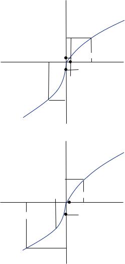

 v
v


 . The larger the losses relative to gains, the more likely the behavior will display risk-loving properties. Moreover, the larger the amounts involved, the more likely the gambler will display risk-loving behavior. With either small amounts involved in the gamble or amounts that are skewed toward gains, the gambler is more likely to display risk-averse behavior. Thus, prospect theory predicts that people display both risk-loving and risk-averse behavior. Which of these behaviors prevails depends upon the size of the stakes involved and whether the gambler is dealing with potential gains or losses, or both. This observation forms the basis for prospect theory analysis of decision under risk.