- •1. INTRODUCTION
- •1.1 BASIC TERMINOLOGY
- •1.2 EXAMPLE SYSTEM
- •1.3 SUMMARY
- •1.4 PRACTICE PROBLEMS
- •2. TRANSLATION
- •2.1 INTRODUCTION
- •2.2 MODELING
- •2.2.1 Free Body Diagrams
- •2.2.2 Mass and Inertia
- •2.2.3 Gravity and Other Fields
- •2.2.4 Springs
- •2.2.5 Damping and Drag
- •2.2.6 Cables And Pulleys
- •2.2.7 Friction
- •2.2.8 Contact Points And Joints
- •2.3 SYSTEM EXAMPLES
- •2.4 OTHER TOPICS
- •2.5 SUMMARY
- •2.6 PRACTICE PROBLEMS
- •2.7 PRACTICE PROBLEM SOLUTIONS
- •2.8 ASSIGNMENT PROBLEMS
- •3. ANALYSIS OF DIFFERENTIAL EQUATIONS
- •3.1 INTRODUCTION
- •3.2 EXPLICIT SOLUTIONS
- •3.3 RESPONSES
- •3.3.1 First-order
- •3.3.2 Second-order
- •3.3.3 Other Responses
- •3.4 RESPONSE ANALYSIS
- •3.5 NON-LINEAR SYSTEMS
- •3.5.1 Non-Linear Differential Equations
- •3.5.2 Non-Linear Equation Terms
- •3.5.3 Changing Systems
- •3.6 CASE STUDY
- •3.7 SUMMARY
- •3.8 PRACTICE PROBLEMS
- •3.9 PRACTICE PROBLEM SOLUTIONS
- •3.10 ASSIGNMENT PROBLEMS
- •4. NUMERICAL ANALYSIS
- •4.1 INTRODUCTION
- •4.2 THE GENERAL METHOD
- •4.2.1 State Variable Form
- •4.3 NUMERICAL INTEGRATION
- •4.3.1 Numerical Integration With Tools
- •4.3.2 Numerical Integration
- •4.3.3 Taylor Series
- •4.3.4 Runge-Kutta Integration
- •4.4 SYSTEM RESPONSE
- •4.4.1 Steady-State Response
- •4.5 DIFFERENTIATION AND INTEGRATION OF EXPERIMENTAL DATA
- •4.6 ADVANCED TOPICS
- •4.6.1 Switching Functions
- •4.6.2 Interpolating Tabular Data
- •4.6.3 Modeling Functions with Splines
- •4.6.4 Non-Linear Elements
- •4.7 CASE STUDY
- •4.8 SUMMARY
- •4.9 PRACTICE PROBLEMS
- •4.10 PRACTICE PROBLEM SOLUTIONS
- •4.11 ASSIGNMENT PROBLEMS
- •5. ROTATION
- •5.1 INTRODUCTION
- •5.2 MODELING
- •5.2.1 Inertia
- •5.2.2 Springs
- •5.2.3 Damping
- •5.2.4 Levers
- •5.2.5 Gears and Belts
- •5.2.6 Friction
- •5.2.7 Permanent Magnet Electric Motors
- •5.3 OTHER TOPICS
- •5.4 DESIGN CASE
- •5.5 SUMMARY
- •5.6 PRACTICE PROBLEMS
- •5.7 PRACTICE PROBLEM SOLUTIONS
- •5.8 ASSIGNMENT PROBLEMS
- •6. INPUT-OUTPUT EQUATIONS
- •6.1 INTRODUCTION
- •6.2 THE DIFFERENTIAL OPERATOR
- •6.3 INPUT-OUTPUT EQUATIONS
- •6.3.1 Converting Input-Output Equations to State Equations
- •6.3.2 Integrating Input-Output Equations
- •6.4 DESIGN CASE
- •6.5 SUMMARY
- •6.6 PRACTICE PROBLEMS
- •6.7 PRACTICE PROBLEM SOLUTIONS
- •6.8 ASSGINMENT PROBLEMS
- •6.9 REFERENCES
- •7. ELECTRICAL SYSTEMS
- •7.1 INTRODUCTION
- •7.2 MODELING
- •7.2.1 Resistors
- •7.2.2 Voltage and Current Sources
- •7.2.3 Capacitors
- •7.2.4 Inductors
- •7.2.5 Op-Amps
- •7.3 IMPEDANCE
- •7.4 EXAMPLE SYSTEMS
- •7.5 ELECTROMECHANICAL SYSTEMS - MOTORS
- •7.5.1 Permanent Magnet DC Motors
- •7.5.2 Induction Motors
- •7.5.3 Brushless Servo Motors
- •7.6 FILTERS
- •7.7 OTHER TOPICS
- •7.8 SUMMARY
- •7.9 PRACTICE PROBLEMS
- •7.10 PRACTICE PROBLEM SOLUTIONS
- •7.11 ASSIGNMENT PROBLEMS
- •8. FEEDBACK CONTROL SYSTEMS
- •8.1 INTRODUCTION
- •8.2 TRANSFER FUNCTIONS
- •8.3 CONTROL SYSTEMS
- •8.3.1 PID Control Systems
- •8.3.2 Manipulating Block Diagrams
- •8.3.3 A Motor Control System Example
- •8.3.4 System Error
- •8.3.5 Controller Transfer Functions
- •8.3.6 Feedforward Controllers
- •8.3.7 State Equation Based Systems
- •8.3.8 Cascade Controllers
- •8.4 SUMMARY
- •8.5 PRACTICE PROBLEMS
- •8.6 PRACTICE PROBLEM SOLUTIONS
- •8.7 ASSIGNMENT PROBLEMS
- •9. PHASOR ANALYSIS
- •9.1 INTRODUCTION
- •9.2 PHASORS FOR STEADY-STATE ANALYSIS
- •9.3 VIBRATIONS
- •9.4 SUMMARY
- •9.5 PRACTICE PROBLEMS
- •9.6 PRACTICE PROBLEM SOLUTIONS
- •9.7 ASSIGNMENT PROBLEMS
- •10. BODE PLOTS
- •10.1 INTRODUCTION
- •10.2 BODE PLOTS
- •10.3 SIGNAL SPECTRUMS
- •10.4 SUMMARY
- •10.5 PRACTICE PROBLEMS
- •10.6 PRACTICE PROBLEM SOLUTIONS
- •10.7 ASSIGNMENT PROBLEMS
- •10.8 LOG SCALE GRAPH PAPER
- •11. ROOT LOCUS ANALYSIS
- •11.1 INTRODUCTION
- •11.2 ROOT-LOCUS ANALYSIS
- •11.3 SUMMARY
- •11.4 PRACTICE PROBLEMS
- •11.5 PRACTICE PROBLEM SOLUTIONS
- •11.6 ASSIGNMENT PROBLEMS
- •12. NONLINEAR SYSTEMS
- •12.1 INTRODUCTION
- •12.2 SOURCES OF NONLINEARITY
- •12.3.1 Time Variant
- •12.3.2 Switching
- •12.3.3 Deadband
- •12.3.4 Saturation and Clipping
- •12.3.5 Hysteresis and Slip
- •12.3.6 Delays and Lags
- •12.4 SUMMARY
- •12.5 PRACTICE PROBLEMS
- •12.6 PRACTICE PROBLEM SOLUTIONS
- •12.7 ASIGNMENT PROBLEMS
- •13. ANALOG INPUTS AND OUTPUTS
- •13.1 INTRODUCTION
- •13.2 ANALOG INPUTS
- •13.3 ANALOG OUTPUTS
- •13.4 NOISE REDUCTION
- •13.4.1 Shielding
- •13.4.2 Grounding
- •13.5 CASE STUDY
- •13.6 SUMMARY
- •13.7 PRACTICE PROBLEMS
- •13.8 PRACTICE PROBLEM SOLUTIONS
- •13.9 ASSIGNMENT PROBLEMS
- •14. CONTINUOUS SENSORS
- •14.1 INTRODUCTION
- •14.2 INDUSTRIAL SENSORS
- •14.2.1 Angular Displacement
- •14.2.1.1 - Potentiometers
- •14.2.2 Encoders
- •14.2.2.1 - Tachometers
- •14.2.3 Linear Position
- •14.2.3.1 - Potentiometers
- •14.2.3.2 - Linear Variable Differential Transformers (LVDT)
- •14.2.3.3 - Moire Fringes
- •14.2.3.4 - Accelerometers
- •14.2.4 Forces and Moments
- •14.2.4.1 - Strain Gages
- •14.2.4.2 - Piezoelectric
- •14.2.5 Liquids and Gases
- •14.2.5.1 - Pressure
- •14.2.5.2 - Venturi Valves
- •14.2.5.3 - Coriolis Flow Meter
- •14.2.5.4 - Magnetic Flow Meter
- •14.2.5.5 - Ultrasonic Flow Meter
- •14.2.5.6 - Vortex Flow Meter
- •14.2.5.7 - Positive Displacement Meters
- •14.2.5.8 - Pitot Tubes
- •14.2.6 Temperature
- •14.2.6.1 - Resistive Temperature Detectors (RTDs)
- •14.2.6.2 - Thermocouples
- •14.2.6.3 - Thermistors
- •14.2.6.4 - Other Sensors
- •14.2.7 Light
- •14.2.7.1 - Light Dependant Resistors (LDR)
- •14.2.8 Chemical
- •14.2.8.2 - Conductivity
- •14.2.9 Others
- •14.3 INPUT ISSUES
- •14.4 SENSOR GLOSSARY
- •14.5 SUMMARY
- •14.6 REFERENCES
- •14.7 PRACTICE PROBLEMS
- •14.8 PRACTICE PROBLEM SOLUTIONS
- •14.9 ASSIGNMENT PROBLEMS
- •15. CONTINUOUS ACTUATORS
- •15.1 INTRODUCTION
- •15.2 ELECTRIC MOTORS
- •15.2.1 Basic Brushed DC Motors
- •15.2.2 AC Motors
- •15.2.3 Brushless DC Motors
- •15.2.4 Stepper Motors
- •15.2.5 Wound Field Motors
- •15.3 HYDRAULICS
- •15.4 OTHER SYSTEMS
- •15.5 SUMMARY
- •15.6 PRACTICE PROBLEMS
- •15.7 PRACTICE PROBLEM SOLUTIONS
- •15.8 ASSIGNMENT PROBLEMS
- •16. MOTION CONTROL
- •16.1 INTRODUCTION
- •16.2 MOTION PROFILES
- •16.2.1 Velocity Profiles
- •16.2.2 Position Profiles
- •16.3 MULTI AXIS MOTION
- •16.3.1 Slew Motion
- •16.3.1.1 - Interpolated Motion
- •16.3.2 Motion Scheduling
- •16.4 PATH PLANNING
- •16.5 CASE STUDIES
- •16.6 SUMMARY
- •16.7 PRACTICE PROBLEMS
- •16.8 PRACTICE PROBLEM SOLUTIONS
- •16.9 ASSIGNMENT PROBLEMS
- •17. LAPLACE TRANSFORMS
- •17.1 INTRODUCTION
- •17.2 APPLYING LAPLACE TRANSFORMS
- •17.2.1 A Few Transform Tables
- •17.3 MODELING TRANSFER FUNCTIONS IN THE s-DOMAIN
- •17.4 FINDING OUTPUT EQUATIONS
- •17.5 INVERSE TRANSFORMS AND PARTIAL FRACTIONS
- •17.6 EXAMPLES
- •17.6.2 Circuits
- •17.7 ADVANCED TOPICS
- •17.7.1 Input Functions
- •17.7.2 Initial and Final Value Theorems
- •17.8 A MAP OF TECHNIQUES FOR LAPLACE ANALYSIS
- •17.9 SUMMARY
- •17.10 PRACTICE PROBLEMS
- •17.11 PRACTICE PROBLEM SOLUTIONS
- •17.12 ASSIGNMENT PROBLEMS
- •17.13 REFERENCES
- •18. CONTROL SYSTEM ANALYSIS
- •18.1 INTRODUCTION
- •18.2 CONTROL SYSTEMS
- •18.2.1 PID Control Systems
- •18.2.2 Analysis of PID Controlled Systems With Laplace Transforms
- •18.2.3 Finding The System Response To An Input
- •18.2.4 Controller Transfer Functions
- •18.3.1 Approximate Plotting Techniques
- •18.4 DESIGN OF CONTINUOUS CONTROLLERS
- •18.5 SUMMARY
- •18.6 PRACTICE PROBLEMS
- •18.7 PRACTICE PROBLEM SOLUTIONS
- •18.8 ASSIGNMENT PROBLEMS
- •19. CONVOLUTION
- •19.1 INTRODUCTION
- •19.2 UNIT IMPULSE FUNCTIONS
- •19.3 IMPULSE RESPONSE
- •19.4 CONVOLUTION
- •19.5 NUMERICAL CONVOLUTION
- •19.6 LAPLACE IMPULSE FUNCTIONS
- •19.7 SUMMARY
- •19.8 PRACTICE PROBLEMS
- •19.9 PRACTICE PROBLEM SOLUTIONS
- •19.10 ASSIGNMENT PROBLEMS
- •20. STATE SPACE ANALYSIS
- •20.1 INTRODUCTION
- •20.2 OBSERVABILITY
- •20.3 CONTROLLABILITY
- •20.4 OBSERVERS
- •20.5 SUMMARY
- •20.6 PRACTICE PROBLEMS
- •20.7 PRACTICE PROBLEM SOLUTIONS
- •20.8 ASSIGNMENT PROBLEMS
- •20.9 BIBLIOGRAPHY
- •21. STATE SPACE CONTROLLERS
- •21.1 INTRODUCTION
- •21.2 FULL STATE FEEDBACK
- •21.3 OBSERVERS
- •21.4 SUPPLEMENTAL OBSERVERS
- •21.5 REGULATED CONTROL WITH OBSERVERS
- •21.7 LINEAR QUADRATIC GAUSSIAN (LQG) COMPENSATORS
- •21.8 VERIFYING CONTROL SYSTEM STABILITY
- •21.8.1 Stability
- •21.8.2 Bounded Gain
- •21.9 ADAPTIVE CONTROLLERS
- •21.10 OTHER METHODS
- •21.10.1 Kalman Filtering
- •21.11 SUMMARY
- •21.12 PRACTICE PROBLEMS
- •21.13 PRACTICE PROBLEM SOLUTIONS
- •21.14 ASSIGNMENT PROBLEMS
- •22. SYSTEM IDENTIFICATION
- •22.1 INTRODUCTION
- •22.2 SUMMARY
- •22.3 PRACTICE PROBLEMS
- •22.4 PRACTICE PROBLEM SOLUTIONS
- •22.5 ASSIGNMENT PROBLEMS
- •23. ELECTROMECHANICAL SYSTEMS
- •23.1 INTRODUCTION
- •23.2 MATHEMATICAL PROPERTIES
- •23.2.1 Induction
- •23.3 EXAMPLE SYSTEMS
- •23.4 SUMMARY
- •23.5 PRACTICE PROBLEMS
- •23.6 PRACTICE PROBLEM SOLUTIONS
- •23.7 ASSIGNMENT PROBLEMS
- •24. FLUID SYSTEMS
- •24.1 SUMMARY
- •24.2 MATHEMATICAL PROPERTIES
- •24.2.1 Resistance
- •24.2.2 Capacitance
- •24.2.3 Power Sources
- •24.3 EXAMPLE SYSTEMS
- •24.4 SUMMARY
- •24.5 PRACTICE PROBLEMS
- •24.6 PRACTICE PROBLEMS SOLUTIONS
- •24.7 ASSIGNMENT PROBLEMS
- •25. THERMAL SYSTEMS
- •25.1 INTRODUCTION
- •25.2 MATHEMATICAL PROPERTIES
- •25.2.1 Resistance
- •25.2.2 Capacitance
- •25.2.3 Sources
- •25.3 EXAMPLE SYSTEMS
- •25.4 SUMMARY
- •25.5 PRACTICE PROBLEMS
- •25.6 PRACTICE PROBLEM SOLUTIONS
- •25.7 ASSIGNMENT PROBLEMS
- •26. OPTIMIZATION
- •26.1 INTRODUCTION
- •26.2 OBJECTIVES AND CONSTRAINTS
- •26.3 SEARCHING FOR THE OPTIMUM
- •26.4 OPTIMIZATION ALGORITHMS
- •26.4.1 Random Walk
- •26.4.2 Gradient Decent
- •26.4.3 Simplex
- •26.5 SUMMARY
- •26.6 PRACTICE PROBLEMS
- •26.7 PRACTICE PROBLEM SOLUTIONS
- •26.8 ASSIGNMENT PROBLEMS
- •27. FINITE ELEMENT ANALYSIS (FEA)
- •27.1 INTRODUCTION
- •27.2 FINITE ELEMENT MODELS
- •27.3 FINITE ELEMENT MODELS
- •27.4 SUMMARY
- •27.5 PRACTICE PROBLEMS
- •27.6 PRACTICE PROBLEM SOLUTIONS
- •27.7 ASSIGNMENT PROBLEMS
- •27.8 BIBLIOGRAPHY
- •28. FUZZY LOGIC
- •28.1 INTRODUCTION
- •28.2 COMMERCIAL CONTROLLERS
- •28.3 REFERENCES
- •28.4 SUMMARY
- •28.5 PRACTICE PROBLEMS
- •28.6 PRACTICE PROBLEM SOLUTIONS
- •28.7 ASSIGNMENT PROBLEMS
- •29. NEURAL NETWORKS
- •29.1 SUMMARY
- •29.2 PRACTICE PROBLEMS
- •29.3 PRACTICE PROBLEM SOLUTIONS
- •29.4 ASSIGNMENT PROBLEMS
- •29.5 REFERENCES
- •30. EMBEDDED CONTROL SYSTEM
- •30.1 INTRODUCTION
- •30.2 CASE STUDY
- •30.3 SUMMARY
- •30.4 PRACTICE PROBLEMS
- •30.5 PRACTICE PROBLEM SOLUTIONS
- •30.6 ASSIGNMENT PROBLEMS
- •31. WRITING
- •31.1 FORGET WHAT YOU WERE TAUGHT BEFORE
- •31.2 WHY WRITE REPORTS?
- •31.3 THE TECHNICAL DEPTH OF THE REPORT
- •31.4 TYPES OF REPORTS
- •31.5 LABORATORY REPORTS
- •31.5.0.1 - An Example First Draft of a Report
- •31.5.0.2 - An Example Final Draft of a Report
- •31.6 RESEARCH
- •31.7 DRAFT REPORTS
- •31.8 PROJECT REPORT
- •31.9 OTHER REPORT TYPES
- •31.9.1 Executive
- •31.9.2 Consulting
- •31.9.3 Memo(randum)
- •31.9.4 Interim
- •31.9.5 Poster
- •31.9.6 Progress Report
- •31.9.7 Oral
- •31.9.8 Patent
- •31.10 LAB BOOKS
- •31.11 REPORT ELEMENTS
- •31.11.1 Figures
- •31.11.2 Graphs
- •31.11.3 Tables
- •31.11.4 Equations
- •31.11.5 Experimental Data
- •31.11.6 Result Summary
- •31.11.7 References
- •31.11.8 Acknowledgments
- •31.11.9 Abstracts
- •31.11.10 Appendices
- •31.11.11 Page Numbering
- •31.11.12 Numbers and Units
- •31.11.13 Engineering Drawings
- •31.11.14 Discussions
- •31.11.15 Conclusions
- •31.11.16 Recomendations
- •31.11.17 Appendices
- •31.11.18 Units
- •31.12 GENERAL WRITING ISSUES
- •31.13 WRITERS BLOCK
- •31.14 TECHNICAL ENGLISH
- •31.15 EVALUATION FORMS
- •31.16 PATENTS
- •32. PROJECTS
- •32.2 OVERVIEW
- •32.2.1 The Objectives and Constraints
- •32.3 MANAGEMENT
- •32.3.1 Timeline - Tentative
- •32.3.2 Teams
- •32.4 DELIVERABLES
- •32.4.1 Conceptual Design
- •32.4.2 EGR 345/101 Contract
- •32.4.3 Progress Reports
- •32.4.4 Design Proposal
- •32.4.5 The Final Report
- •32.5 REPORT ELEMENTS
- •32.5.1 Gantt Charts
- •32.5.2 Drawings
- •32.5.3 Budgets and Bills of Material
- •32.5.4 Calculations
- •32.6 APPENDICES
- •32.6.1 Appendix A - Sample System
- •32.6.2 Appendix B - EGR 345/101 Contract
- •32.6.3 Appendix C - Forms
- •33. ENGINEERING PROBLEM SOLVING
- •33.1 BASIC RULES OF STYLE
- •33.2 EXPECTED ELEMENTS
- •33.3 SEPCIAL ELEMENTS
- •33.3.1 Graphs
- •33.3.2 EGR 345 Specific
- •33.4 SCILAB
- •33.5 TERMINOLOGY
- •34. MATHEMATICAL TOOLS
- •34.1 INTRODUCTION
- •34.1.1 Constants and Other Stuff
- •34.1.2 Basic Operations
- •34.1.2.1 - Factorial
- •34.1.3 Exponents and Logarithms
- •34.1.4 Polynomial Expansions
- •34.1.5 Practice Problems
- •34.2 FUNCTIONS
- •34.2.1 Discrete and Continuous Probability Distributions
- •34.2.2 Basic Polynomials
- •34.2.3 Partial Fractions
- •34.2.4 Summation and Series
- •34.2.5 Practice Problems
- •34.3 SPATIAL RELATIONSHIPS
- •34.3.1 Trigonometry
- •34.3.2 Hyperbolic Functions
- •34.3.2.1 - Practice Problems
- •34.3.3 Geometry
- •34.3.4 Planes, Lines, etc.
- •34.3.5 Practice Problems
- •34.4 COORDINATE SYSTEMS
- •34.4.1 Complex Numbers
- •34.4.2 Cylindrical Coordinates
- •34.4.3 Spherical Coordinates
- •34.4.4 Practice Problems
- •34.5 MATRICES AND VECTORS
- •34.5.1 Vectors
- •34.5.2 Dot (Scalar) Product
- •34.5.3 Cross Product
- •34.5.4 Triple Product
- •34.5.5 Matrices
- •34.5.6 Solving Linear Equations with Matrices
- •34.5.7 Practice Problems
- •34.6 CALCULUS
- •34.6.1 Single Variable Functions
- •34.6.1.1 - Differentiation
- •34.6.1.2 - Integration
- •34.6.2 Vector Calculus
- •34.6.3 Differential Equations
- •34.6.3.1.1 - Guessing
- •34.6.3.1.2 - Separable Equations
- •34.6.3.1.3 - Homogeneous Equations and Substitution
- •34.6.3.2.1 - Linear Homogeneous
- •34.6.3.2.2 - Nonhomogeneous Linear Equations
- •34.6.3.3 - Higher Order Differential Equations
- •34.6.3.4 - Partial Differential Equations
- •34.6.4 Other Calculus Stuff
- •34.6.5 Practice Problems
- •34.7 NUMERICAL METHODS
- •34.7.1 Approximation of Integrals and Derivatives from Sampled Data
- •34.7.3 Taylor Series Integration
- •34.8 LAPLACE TRANSFORMS
- •34.8.1 Laplace Transform Tables
- •34.9 z-TRANSFORMS
- •34.10 FOURIER SERIES
- •34.11 TOPICS NOT COVERED (YET)
- •34.12 REFERENCES/BIBLIOGRAPHY
- •35. A BASIC INTRODUCTION TO ‘C’
- •35.2 BACKGROUND
- •35.3 PROGRAM PARTS
- •35.4 HOW A ‘C’ COMPILER WORKS
- •35.5 STRUCTURED ‘C’ CODE
- •35.7 CREATING TOP DOWN PROGRAMS
- •35.8 HOW THE BEAMCAD PROGRAM WAS DESIGNED
- •35.8.1 Objectives:
- •35.8.2 Problem Definition:
- •35.8.3 User Interface:
- •35.8.3.1 - Screen Layout (also see figure):
- •35.8.3.2 - Input:
- •35.8.3.3 - Output:
- •35.8.3.4 - Help:
- •35.8.3.5 - Error Checking:
- •35.8.3.6 - Miscellaneous:
- •35.8.4 Flow Program:
- •35.8.5 Expand Program:
- •35.8.6 Testing and Debugging:
- •35.8.7 Documentation
- •35.8.7.1 - Users Manual:
- •35.8.7.2 - Programmers Manual:
- •35.8.8 Listing of BeamCAD Program.
- •35.9 PRACTICE PROBLEMS
- •36. UNITS AND CONVERSIONS
- •36.1 HOW TO USE UNITS
- •36.2 HOW TO USE SI UNITS
- •36.3 THE TABLE
- •36.4 ASCII, HEX, BINARY CONVERSION
- •36.5 G-CODES
- •37. ATOMIC MATERIAL DATA
- •37. MECHANICAL MATERIAL PROPERTIES
- •37.1 FORMULA SHEET
- •38. BIBLIOGRAPHY
- •38.1 TEXTBOOKS
- •38.1.1 Slotine and Li
- •38.1.2 VandeVegte
- •39. TOPICS IN DEVELOPMENT
- •39.1 UPDATED DC MOTOR MODEL
- •39.2 ANOTHER DC MOTOR MODEL
- •39.3 BLOCK DIAGRAMS AND UNITS
- •39.4 SIGNAL FLOW GRAPHS
- •39.5 ZERO ORDER HOLD
- •39.6 TORSIONAL DAMPERS
- •39.7 MISC
- •39.8 Nyquist Plot
- •39.9 NICHOLS CHART
- •39.10 BESSEL POLYNOMIALS
- •39.11 ITAE
- •39.12 ROOT LOCUS
- •39.13 LYAPUNOV’S LINEARIZATION METHOD
- •39.14 XXXXX
- •39.15 XXXXX
- •39.16 XXXXX
- •39.17 XXXXX
- •39.18 XXXXX
- •39.19 XXXXX
- •39.20 XXXXX
- •39.21 SUMMARY
- •39.22 PRACTICE PROBLEMS
- •39.23 PRACTICE PROBLEM SOLUTIONS
- •39.24 ASSGINMENT PROBLEMS
- •39.25 REFERENCES
- •39.26 BIBLIOGRAPHY
analog IO - 13.1
13. ANALOG INPUTS AND OUTPUTS
Topics:
•Analog inputs and outputs
•Sampling issues; aliasing, quantization error, resolution
Objectives:
•To understand the basics of conversion to and from analog values.
13.1INTRODUCTION
An analog value is continuous, not discrete, as shown in Figure 13.1. In the previous chapters, techniques were discussed for designing continuos control systems. In this chapter we will examine analog inputs and outputs so that we may design continuous control systems that use computers.
Voltage |
logical |
continuous |
t |
Figure 13.1 Logical and Continuous Values
Typical analog inputs and outputs for computers are listed below. Actuators and sensors that can be used with analog inputs and outputs will be discussed in later chapters.
Inputs:
•oven temperature
•fluid pressure
•fluid flow rate
Outputs:
analog IO - 13.2
•fluid valve position
•motor position
•motor velocity
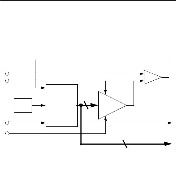
A basic analog input is shown in Figure 13.2. In this type of system a physical value is converted to a voltage, current or other value by a transducer. A signal conditioner converts the signal from the transducer to a voltage or current that is read by the analog input.
physical |
|
|
transducer |
|
|
signal |
|
|
analog |
|
integer |
|
|
|
|
||||||||
phenomenon |
(ie., sensor) |
|
|
conditioning |
|
|
input |
|
|
||
|
|
|
|
|
|
|
|
|
|
|
|
Figure 13.2 Analog inputs
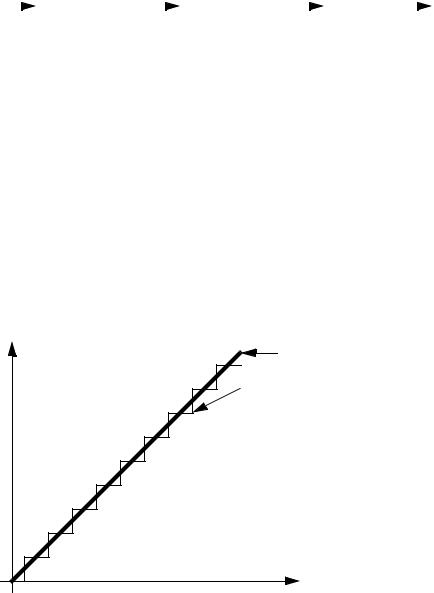
Analog to digital and digital to analog conversion uses integers within the computer. Integers limit the resolution of the numbers to a discrete, or quantized range. The effect of using integers is shown in Figure 13.3 where the desired or actual analog value is continuous, but the possible integer values are quantified with a ’staircase’ set of values. Consider when a continuous analog voltage is being read, it must be quantized into an available integer value. Likewise, a desired analog output value is limited to available quantized values. In general the difference between the analog and quantized integer value is an error based upon the resolution of the analog I/O.
analog |
continuous |
|
|
|
quantized |
|
integer |
analog IO - 13.3
Figure 13.3 Quantization error
13.2 ANALOG INPUTS
To input an analog voltage (into a computer) the continuous voltage value must be sampled and then converted to a numerical value by an A/D (Analog to Digital) converter (also known as ADC). Figure 13.4 shows a continuous voltage changing over time. There are three samples shown on the figure. The process of sampling the data is not instantaneous, so each sample has a start and stop time. The time required to acquire the sample is called the sampling time. A/D converters can only acquire a limited number of samples per second. The time between samples is called the sampling period T, and the inverse of the sampling period is the sampling frequency (also called sampling rate). The sampling time is often much smaller than the sampling period. The sampling frequency is specified when buying hardware, but a common sampling rate is 100KHz.
Voltage is sampled during these time periods
voltage |
|
|
time |
T = (Sampling Frequency)-1 |
Sampling time |
Figure 13.4 Sampling an Analog Voltage
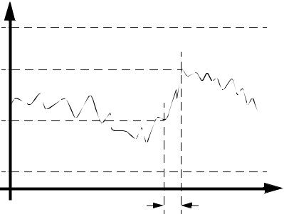
A more realistic drawing of sampled data is shown in Figure 13.5. This data is noisier, and even between the start and end of the data sample there is a significant change in the voltage value. The data value sampled will be somewhere between the voltage at the start and end of the sample. The maximum (Vmax) and minimum (Vmin) voltages are a function of the control hardware. These are often specified when purchasing hardware, but reasonable ranges are;
analog IO - 13.4
0V to 5V
0V to 10V -5V to 5V -10V to 10V
The number of bits of the A/D converter is the number of bits in the result word. If the A/D converter is 8 bit then the result can read up to 256 different voltage levels. Most A/D converters have 12 bits, 16 bit converters are used for precision measurements.
V( t) |
|
|
|
|
|
|
|
|
|
|
|
|
Vmax |
V( t2) |
|
|
|
|
|
|
V( t1) |
|
|
|
|
|
|
|
|
|
|
|
|
Vmin |
|
|
|
|
|
|
t |
|
|
|
|
|
|
τ |
where, |
|
|
|
|
t1 |
t2 |
V( t) |
= |
the actual voltage over time |
||||
τ |
= |
sample interval for A/D converter |
||||
t |
= |
time |
|
|
|
|
t1, t2 = |
time at start,end of sample |
|||||
V( t1) , V( t2) |
= |
voltage at start, end of sample |
Vmin, Vmax = input voltage range of A/D converter
N = number of bits in the A/D converter
Figure 13.5 Parameters for an A/D Conversion
The parameters defined in Figure 13.5 can be used to calculate values for A/D converters. These equations are summarized in Figure 13.6. Equation 1 relates the number of
analog IO - 13.5
bits of an A/D converter to the resolution. Equation 2 gives the error that can be expected with an A/D converter given the range between the minimum and maximum voltages, and the resolution (this is commonly called the quantization error). Equation 3 relates the voltage range and resolution to the voltage input to estimate the integer that the A/D converter will record. Finally, equation 4 allows a conversion between the integer value from the A/ D converter, and a voltage in the computer.
R = 2 |
N |
|
|
|
|
|
|
|
|
(1) |
||||
|
|
|
|
|
|
|
|
|
|
|
||||
V |
|
|
|
|
= |
|
± |
Vmax – Vmin |
(2) |
|||||
|
|
|
|
|
---------------------------- |
|
||||||||
|
ERROR |
|
|
|
|
2R |
|
|
||||||
|
|
|
|
|
|
|
|
|
|
|
||||
|
|
|
|
|
|
|
Vin – Vmin |
|
|
|
|
|||
VI |
= |
INT |
|
( R – 1) |
|
(3) |
||||||||
|
---------------------------- |
|
||||||||||||
|
|
|
|
|
|
|
V |
|
– V |
|
|
|
|
|
|
|
|
|
|
|
|
|
max |
|
min |
|
|
|
|
|
|
|
|
|
VI |
|
|
|
|
|
||||
VC |
= |
|
( Vmax – Vmin) + Vmin |
(4) |
||||||||||
|
----------- |
|||||||||||||
|
|
|
|
R – 1 |
|
|
|
|
|
|
|
where,
R = resolution of A/D converter
VI = the integer value representing the input voltage
VC = the voltage calculated from the integer value
VERROR = the maximum quantization error
Figure 13.6 A/D Converter Equations
Consider a simple example, a 10 bit A/D converter can read voltages between - 10V and 10V. This gives a resolution of 1024, where 0 is -10V and 1023 is +10V. Because there are only 1024 steps there is a maximum error of ±9.8mV. If a voltage of 4.564V is input into the PLC, the A/D converter converts the voltage to an integer value of 746. When we convert this back to a voltage the result is 4.570V. The resulting quantization error is 4.570V-4.564V=+0.006V. This error can be reduced by selecting an A/D converter with more bits. Each bit halves the quantization error.
analog IO - 13.6
Given,
N = 10
Vmax = 10V
Vmin = –10V
Vin = 4.564V
Calculate,
R = 2N = 1024
|
|
|
|
|
|
|
|
|
|
|
|
|
|
|
|
|
|
|
|
|
|
|
|
|
|
|
|
|
Vmax |
– Vmin |
|
|
|
|
|
|
|
|
|
|
|
|
|
|
|
|
|
|
|
|
|
|
|
|
|
|
|
|
|
|
|
|
|
|
|
|
|
|
||||||||||||
|
|
|
|
|
|
|
|
|
|
|
|
|
|
|
|
|
|
|
|
|
|
|
|
|
|
|
|
|
|
|
|
|
|
|
|
|
|
|
|
|
|
|
|
|
|
|
|
|
|
|
|
|
|
|
|
|
|
|
|
|
|
|
|
|
|
|
||||||||||||||
|
|
|
|
|
|
|
|
|
|
|
|
|
|
|
|
|
|
|
|
|
|
|
|
|
|
|
|
|
|
|
|
|
|
|
|
|
|
|
|
|
|
|
|
|
|
|
|
|
|
|
|
|
|
|
|
|
|
|
|
|
|
|
|
|
|
|
||||||||||||||
|
|
|
|
|
|
|
|
|
|
|
|
|
|
|
|
|
|
|
|
|
|
|
|
|
|
|
|
|
|
|
|
|
|
|
|
|
|
|
|
|
|
|
|
|
|
|
|
|
|
|
|
|
|
|
|
|
|
|
|
|
|
|
|
|
|
|
||||||||||||||
|
|
|
|
|
|
|
|
|
|
|
|
|
|
VERROR = |
|
---------------------------- |
= |
0.0098V |
|
|||||||||||||||||||||||||||||||||||||||||||||||||||||||||||||
|
|
|
|
|
|
|
|
|
|
|
|
|
|
|
||||||||||||||||||||||||||||||||||||||||||||||||||||||||||||||||||
|
|
|
|
|
|
|
|
|
|
|
|
|
|
|
|
|
|
|
|
|
|
|
|
|
|
|
|
|
|
|
|
|
2R |
|
|
|
|
|
|
|
|
|
|
|
|
|
|
|
|
|
|
|
|
|
|
|
|
|
|
|
|
|
|
|
|
|
|
|
|
|
|
|
|
|
|
|||||
|
|
|
|
|
|
|
|
|
|
|
|
|
|
|
|
|
|
|
|
|
|
|
|
|
|
|
|
|
|
|
|
|
|
|
|
|
|
|
|
|
|
|
|
|
|
|
|
|
|
|
|
|
|
|
|
|
|
|
|
|
|
|
|
|
|
|
|
|
|
|
|
|
||||||||
|
|
|
|
|
|
|
|
|
|
|
|
|
|
|
|
|
|
|
|
|
|
|
|
|
|
|
|
Vin |
– Vmin |
|
|
|
|
|
|
|
|
|
|
|
|
|
|
|
|
|
|
|
|
|
|
|
|
|
|
|
|
|
|
|
|
|
|
|
|
|
|
|
||||||||||||
|
|
|
|
|
|
|
|
|
|
|
|
|
|
|
|
|
|
|
|
|
|
|
|
|
|
|
|
|
|
|
|
|
|
|
|
|
|
|
|
|
|
|
|
|
|
|
|
|
|
|
|
|
|
|
|
|
|
|
|
|
|
|
|
|
||||||||||||||||
|
|
|
|
|
|
|
|
|
|
|
|
|
|
|
|
|
|
|
|
|
|
|
|
|
|
|
|
|
|
|
|
|
|
|
|
|
|
|
|
|
|
|
|
|
|
|
|
|
|
|
|
|
|
|
|
|
|
|
|
|
|
|
|
|
||||||||||||||||
|
|
|
|
|
|
|
|
|
|
|
|
|
|
|
|
|
|
|
|
|
|
|
|
|
|
|
|
|
|
|
|
|
|
|
|
|
|
|
|
|
|
|
|
|
|
|
|
|
|
|
|
|
|
|
|
|
|
|
|
|
|
|
|
|
||||||||||||||||
|
|
|
|
|
|
|
|
|
|
|
|
|
|
VI |
= |
|
INT |
|
|
---------------------------- |
|
R |
|
= 746 |
|
|
|
|
|
|
|
|
|
|
|
|
|
|
|
|
|
|
|
|
|
|
|
|
|
|
|
|
||||||||||||||||||||||||||||
|
|
|
|
|
|
|
|
|
|
|
|
|
|
|
|
|
|
|
|
|
|
|
|
|
|
|
V |
|
|
|
|
– V |
|
|
|
|
|
|
|
|
|
|
|
|
|
|
|
|
|
|
|
|
|
|
|
|
|
|
|
|
|
|
|
|
|
|
|
|
|
|
|
|
|
|||||||
|
|
|
|
|
|
|
|
|
|
|
|
|
|
|
|
|
|
|
|
|
|
|
|
|
|
|
|
|
|
|
|
|
|
|
|
|
|
|
|
|
|
|
|
|
|
|
|
|
|
|
|
|
|
|
|
|
|
|
|
|
|
|
|
|
|
|
|
|
|
|
||||||||||
|
|
|
|
|
|
|
|
|
|
|
|
|
|
|
|
|
|
|
|
|
|
|
|
|
|
|
|
|
|
|
max |
|
|
|
|
min |
|
|
|
|
|
|
|
|
|
|
|
|
|
|
|
|
|
|
|
|
|
|
|
|
|
|
|
|
|
|
|
|
|
|
|
|
|
|
||||||
|
|
|
|
|
|
|
|
|
|
|
|
|
|
|
|
|
|
|
|
|
|
VI |
|
|
|
|
|
|
|
|
|
|
|
|
|
|
|
|
|
|
|
|
|
|
|
|
|
|
|
|
|
|
|
|
|
|
|
|
|
|
|
|
|
|
|
|
|
|
||||||||||||
|
|
|
|
|
|
|
|
|
|
|
|
|
|
|
|
|
|
|
|
|
|
|
|
|
|
|
|
|
|
|
|
|
|
|
|
|
|
|
|
|
|
|
|
|
|
|
|
|
|
|
|
|
|
|
|
|
|
|
|
|
|
|
|
|
|
|
|
|
|
|
|
|
|
|
|
|||||
|
|
|
|
|
|
|
|
|
|
|
|
|
|
|
|
|
|
|
|
|
|
|
|
|
|
|
|
|
|
|
|
|
|
|
|
|
|
|
|
|
|
|
|
|
|
|
|
|
|
|
|
|
|
|
|
|
|
|
|
|
|
|
|
|
|
|
|
|
|
|
|
|
|
|
|
|||||
|
|
|
|
|
|
|
|
|
|
|
|
|
|
|
|
|
|
|
|
|
|
|
|
|
|
|
|
|
|
|
|
|
|
|
|
|
|
|
|
|
|
|
|
|
|
|
|
|
|
|
|
|
|
|
|
|
|
|
|
|
|
|
|
|
|
|
|
|
|
|
|
|
|
|
|
|||||
|
|
|
|
|
|
|
|
|
|
|
|
|
|
V |
= |
|
---- |
( V |
|
|
|
|
|
– V |
|
|
|
) |
|
+ V |
|
|
|
= 4.570V |
|
|||||||||||||||||||||||||||||||||||||||||||||
|
|
|
|
|
|
|
|
|
|
|
|
|
|
|
|
|
|
|
|
|
|
|
|
|
|
|||||||||||||||||||||||||||||||||||||||||||||||||||||||
|
|
|
|
|
|
|
|
|
|
|
|
|
|
|
C |
|
|
|
|
|
R |
|
|
|
max |
|
|
|
|
min |
|
|
|
|
|
|
min |
|
|
|
|
|
|
|
|
|
|
|
|
|
|
|
|
|
|
|
|
|
|
|
|
|
|
|
|
|
|
|
||||||||||||
|
|
|
|
|
|
|
|
|
|
|
|
|
|
|
|
|
|
|
|
|
|
|
|
|
|
|
|
|
|
|
|
|
|
|
|
|
|
|
|
|
|
|
|
|
|
|
|
|
|
|
|
|
|
|
|
|
|
|
|
|
|
|
|
|
|
|
|
|
|
|
|
|
|
|
|
|
|
|
|
|
Figure 13.7 Sample Calculation of A/D Values
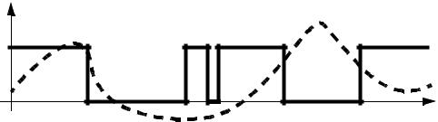
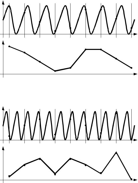
If the voltage being sampled is changing too fast we may get false readings, as shown in Figure 13.8. In the upper graph the waveform completes seven cycles, and 9 samples are taken. The bottom graph plots out the values read. The sampling frequency was too low, so the signal read appears to be different that it actually is, this is called aliasing.
analog IO - 13.7
Figure 13.8 Low Sampling Frequencies Cause Aliasing
Figure 13.9 Very Low Sampling Frequencies Produce Apparently Random
The Nyquist criterion specifies that sampling frequencies should be at least twice the frequency of the signal being measured, otherwise aliasing will occur. The example in
analog IO - 13.8
Figure 13.8 violated this principle, so the signal was aliased. If this happens in real applications the process will appear to operate erratically. In practice the sample frequency should be 4 or more times faster than the system frequency.
fAD > 2fsignal |
where, |
|
fAD = sampling frequency |
|
fsignal = maximum frequency of the input |
There are other practical details that should be considered when designing applications with analog inputs;
•Noise - Since the sampling window for a signal is short, noise will have added effect on the signal read. For example, a momentary voltage spike might result in a higher than normal reading. Shielded data cables are commonly used to reduce the noise levels.
•Delay - When the sample is requested, a short period of time passes before the final sample value is obtained.
•Multiplexing - Most analog input cards allow multiple inputs. These may share the A/D converter using a technique called multiplexing. If there are 4 channels using an A/D converter with a maximum sampling rate of 100Hz, the maximum sampling rate per channel is 25Hz.
•Signal Conditioners - Signal conditioners are used to amplify, or filter signals coming from transducers, before they are read by the A/D converter.
•Resistance - A/D converters normally have high input impedance (resistance), so they affect circuits they are measuring.
•Single Ended Inputs - Voltage inputs to a PLC can use a single common for multiple inputs, these types of inputs are called single ended inputs. These tend to be more prone to noise.
•Double Ended Inputs - Each double ended input has its own common. This reduces problems with electrical noise, but also tends to reduce the number of inputs by half.
•Sampling Rates - The maximum number of samples that can be read each second. If reading multiple channels with a multiplexer, this may be reduced.
•Quantization Error - Analog IO is limited by the binary resolution of the converter. This means that the output is at discrete levels, instead of continuous values.
•Triggers - often external digital signals are used to signal the start of data collection.
•Range - the typical voltages that the card can read. Typical voltage ranges are - 10V to 10V, 0V to 10V, 0V to 5V, 1V to 5V, -5V to 5V, 4mA to 20mA.
•DMA - a method to write large blocks of memory directly to computer memory. This is normally used for high speed data captures.
analog IO - 13.9
•Filters - some A/D input cards will provide built in functions to filter the incoming data to remove high frequency noise components.
•Input impedance - most analog inputs have very high input resistances, in the range of Mohms.
ASIDE: This device is an 8 bit A/D converter. The main concept behind this is the successive approximation logic. Once the reset is toggled the converter will start by setting the most significant bit of the 8 bit number. This will be converted to a voltage Ve that is a function of the +/-Vref values. The value of Ve is compared to Vin and a simple logic check determines which is larger. If the value of Ve is larger the bit is turned off. The logic then repeats similar steps from the most to least significant bits. Once the last bit has been set on/off and checked the conversion will be complete, and a done bit can be set to indicate a valid conversion value.
Vin above (+ve) or below (-ve) Ve
Vin |
+ |
- |
+Vref |
|
successive |
8 |
|
|
clock |
approximation |
D to A |
|
|
converter |
|
|||
logic |
Ve |
|||
|
||||
|
|
|||
reset |
|
|
done |
|
-Vref |
|
|
8 |
|
|
|
data out |
||
|
|
|
Quite often an A/D converter will multiplex between various inputs. As it switches the voltage will be sampled by a sample and hold circuit. This will then be converted to a digital value. The sample and hold circuits can be used before the multiplexer to collect data values at the same instant in time.
Figure 13.10 A Successive Approximation A/D Converter