k-means can be paired with another algorithm to describe non-convex clusters. One first clusters the data into a large number of groups using k-means. These groups are then agglomerated into larger clusters using single link hierarchical clustering, which can detect complex shapes. This approach also makes the solution less sensitive to initialization, and since the hierarchical method provides results at multiple resolutions, one does not need to pre-specify k either.

The cost of the optimal solution decreases with increasing k till it hits zero when the number of clusters equals the number of distinct data-points. This makes it more difficult to (a) directly compare solutions with different numbers of clusters and (b) to find the optimum value of k. If the desired k is not known in advance, one will typically run k-means with different values of k, and then use a suitable criterion to select one of the results. For example, SAS uses the cube-clustering-criterion, while X-means adds a complexity term (which increases with k) to the original cost function (Eq. 1) and then identifies the k which minimizes this adjusted cost. Alternatively, one can progressively increase the number of clusters, in conjunction with a suitable stopping criterion. Bisecting k-means [73] achieves this by first putting all the data into a single cluster, and then recursively splitting the least compact cluster into two using 2-means. The celebrated LBG algorithm [34] used for vector quantization doubles the number of clusters till a suitable code-book size is obtained. Both these approaches thus alleviate the need to know k beforehand.

The algorithm is also sensitive to the presence of outliers, since “mean” is not a robust statistic. A preprocessing step to remove outliers can be helpful. Post-processing the results, for example to eliminate small clusters, or to merge close clusters into a large cluster, is also desirable. Ball and Hall’s ISODATA algorithm from 1967 effectively used both preand post-processing on k-means.

2.3 Generalizations and connections

As mentioned earlier, k-means is closely related to fitting a mixture of k isotropic Gaussians to the data. Moreover, the generalization of the distance measure to all Bregman divergences is related to fitting the data with a mixture of k components from the exponential family of distributions. Another broad generalization is to view the “means” as probabilistic models instead of points in Rd . Here, in the assignment step, each data point is assigned to the most likely model to have generated it. In the “relocation” step, the model parameters are updated to best fit the assigned datasets. Such model-based k-means allow one to cater to more complex data, e.g. sequences described by Hidden Markov models.

One can also “kernelize” k-means [19]. Though boundaries between clusters are still linear in the implicit high-dimensional space, they can become non-linear when projected back to the original space, thus allowing kernel k-means to deal with more complex clusters. Dhillon et al. [19] have shown a close connection between kernel k-means and spectral clustering. The K-medoid algorithm is similar to k-means except that the centroids have to belong to the data set being clustered. Fuzzy c-means is also similar, except that it computes fuzzy membership functions for each clusters rather than a hard one.

Despite its drawbacks, k-means remains the most widely used partitional clustering algorithm in practice. The algorithm is simple, easily understandable and reasonably scalable, and can be easily modified to deal with streaming data. To deal with very large datasets, substantial effort has also gone into further speeding up k-means, most notably by using kd-trees or exploiting the triangular inequality to avoid comparing each data point with all the centroids during the assignment step. Continual improvements and generalizations of the

123

basic algorithm have ensured its continued relevance and gradually increased its effectiveness as well.

3 Support vector machines

In today’s machine learning applications, support vector machines (SVM) [83] are considered a must try—it offers one of the most robust and accurate methods among all well-known algorithms. It has a sound theoretical foundation, requires only a dozen examples for training, and is insensitive to the number of dimensions. In addition, efficient methods for training SVM are also being developed at a fast pace.

In a two-class learning task, the aim of SVM is to find the best classification function to distinguish between members of the two classes in the training data. The metric for the concept of the “best” classification function can be realized geometrically. For a linearly separable dataset, a linear classification function corresponds to a separating hyperplane f (x) that passes through the middle of the two classes, separating the two. Once this function is determined, new data instance xn can be classified by simply testing the sign of the function f (xn ); xn belongs to the positive class if f (xn ) > 0.

Because there are many such linear hyperplanes, what SVM additionally guarantee is that the best such function is found by maximizing the margin between the two classes. Intuitively, the margin is defined as the amount of space, or separation between the two classes as defined by the hyperplane. Geometrically, the margin corresponds to the shortest distance between the closest data points to a point on the hyperplane. Having this geometric definition allows us to explore how to maximize the margin, so that even though there are an infinite number of hyperplanes, only a few qualify as the solution to SVM.

The reason why SVM insists on finding the maximum margin hyperplanes is that it offers the best generalization ability. It allows not only the best classification performance (e.g., accuracy) on the training data, but also leaves much room for the correct classification of the future data. To ensure that the maximum margin hyperplanes are actually found, an SVM classifier attempts to maximize the following function with respect to w and b:

where t is the number of training examples, and αi , i = 1, . . . , t, are non-negative numbers such that the derivatives of L P with respect to αi are zero. αi are the Lagrange multipliers and L P is called the Lagrangian. In this equation, the vectors w and constant b define the hyperplane.

There are several important questions and related extensions on the above basic formulation of support vector machines. We list these questions and extensions below.

1.Can we understand the meaning of the SVM through a solid theoretical foundation?

2.Can we extend the SVM formulation to handle cases where we allow errors to exist, when even the best hyperplane must admit some errors on the training data?

3.Can we extend the SVM formulation so that it works in situations where the training data are not linearly separable?

4.Can we extend the SVM formulation so that the task is to predict numerical values or to rank the instances in the likelihood of being a positive class member, rather than classification?

123

5.Can we scale up the algorithm for finding the maximum margin hyperplanes to thousands and millions of instances?

Question 1 Can we understand the meaning of the SVM through a solid theoretical foundation?

Several important theoretical results exist to answer this question.

A learning machine, such as the SVM, can be modeled as a function class based on some parameters α. Different function classes can have different capacity in learning, which is represented by a parameter h known as the VC dimension [83]. The VC dimension measures the maximum number of training examples where the function class can still be used to learn perfectly, by obtaining zero error rates on the training data, for any assignment of class labels on these points. It can be proven that the actual error on the future data is bounded by a sum of two terms. The first term is the training error, and the second term if proportional to the square root of the VC dimension h. Thus, if we can minimize h, we can minimize the future error, as long as we also minimize the training error. In fact, the above maximum margin function learned by SVM learning algorithms is one such function. Thus, theoretically, the SVM algorithm is well founded.

Question 2 Can we extend the SVM formulation to handle cases where we allow errors to exist, when even the best hyperplane must admit some errors on the training data?

To answer this question, imagine that there are a few points of the opposite classes that cross the middle. These points represent the training error that existing even for the maximum margin hyperplanes. The “soft margin” idea is aimed at extending the SVM algorithm [83] so that the hyperplane allows a few of such noisy data to exist. In particular, introduce a slack variable ξi to account for the amount of a violation of classification by the function f (xi ); ξi has a direct geometric explanation through the distance from a mistakenly classified data instance to the hyperplane f (x). Then, the total cost introduced by the slack variables can be used to revise the original objective minimization function.

Question 3 Can we extend the SVM formulation so that it works in situations where the training data are not linearly separable?

The answer to this question depends on an observation on the objective function where the only appearances of xi is in the form of a dot product. Thus, if we extend the dot product xi · xj through a functional mapping (xi) of each xi to a different space H of larger and even possibly infinite dimensions, then the equations still hold. In each equation, where we had the dot product xi · xj, we now have the dot product of the transformed vectors (xi) · (xj), which is called a kernel function.

The kernel function can be used to define a variety of nonlinear relationship between its inputs. For example, besides linear kernel functions, you can define quadratic or exponential kernel functions. Much study in recent years have gone into the study of different kernels for SVM classification [70] and for many other statistical tests. We can also extend the above descriptions of the SVM classifiers from binary classifiers to problems that involve more than two classes. This can be done by repeatedly using one of the classes as a positive class, and the rest as the negative classes (thus, this method is known as the one-against-all method).

Question 4 Can we extend the SVM formulation so that the task is to learn to approximate data using a linear function, or to rank the instances in the likelihood of being a positive class member, rather a classification?

123

SVM can be easily extended to perform numerical calculations. Here we discuss two such extensions. The first is to extend SVM to perform regression analysis, where the goal is to produce a linear function that can approximate that target function. Careful consideration goes into the choice of the error models; in support vector regression, or SVR, the error is defined to be zero when the difference between actual and predicted values are within a epsilon amount. Otherwise, the epsilon insensitive error will grow linearly. The support vectors can then be learned through the minimization of the Lagrangian. An advantage of support vector regression is reported to be its insensitivity to outliers.

Another extension is to learn to rank elements rather than producing a classification for individual elements [39]. Ranking can be reduced to comparing pairs of instances and producing a +1 estimate if the pair is in the correct ranking order, and −1 otherwise. Thus, a way to reduce this task to SVM learning is to construct new instances for each pair of ranked instance in the training data, and to learn a hyperplane on this new training data.

This method can be applied to many areas where ranking is important, such as in document ranking in information retrieval areas.

Question 5 Can we scale up the algorithm for finding the maximum margin hyperplanes to thousands and millions of instances?

One of the initial drawbacks of SVM is its computational inefficiency. However, this problem is being solved with great success. One approach is to break a large optimization problem into a series of smaller problems, where each problem only involves a couple of carefully chosen variables so that the optimization can be done efficiently. The process iterates until all the decomposed optimization problems are solved successfully. A more recent approach is to consider the problem of learning an SVM as that of finding an approximate minimum enclosing ball of a set of instances.

These instances, when mapped to an N -dimensional space, represent a core set that can be used to construct an approximation to the minimum enclosing ball. Solving the SVM learning problem on these core sets can produce a good approximation solution in very fast speed. For example, the core-vector machine [81] thus produced can learn an SVM for millions of data in seconds.

4 The Apriori algorithm

4.1 Description of the algorithm

One of the most popular data mining approaches is to find frequent itemsets from a transaction dataset and derive association rules. Finding frequent itemsets (itemsets with frequency larger than or equal to a user specified minimum support) is not trivial because of its combinatorial explosion. Once frequent itemsets are obtained, it is straightforward to generate association rules with confidence larger than or equal to a user specified minimum confidence.

Apriori is a seminal algorithm for finding frequent itemsets using candidate generation [1]. It is characterized as a level-wise complete search algorithm using anti-monotonicity of itemsets, “if an itemset is not frequent, any of its superset is never frequent”. By convention, Apriori assumes that items within a transaction or itemset are sorted in lexicographic order. Let the set of frequent itemsets of size k be Fk and their candidates be Ck . Apriori first scans the database and searches for frequent itemsets of size 1 by accumulating the count for each item and collecting those that satisfy the minimum support requirement. It then iterates on the following three steps and extracts all the frequent itemsets.

123

1.Generate Ck+1, candidates of frequent itemsets of size k + 1, from the frequent itemsets of size k.

2.Scan the database and calculate the support of each candidate of frequent itemsets.

3.Add those itemsets that satisfies the minimum support requirement to Fk+1.

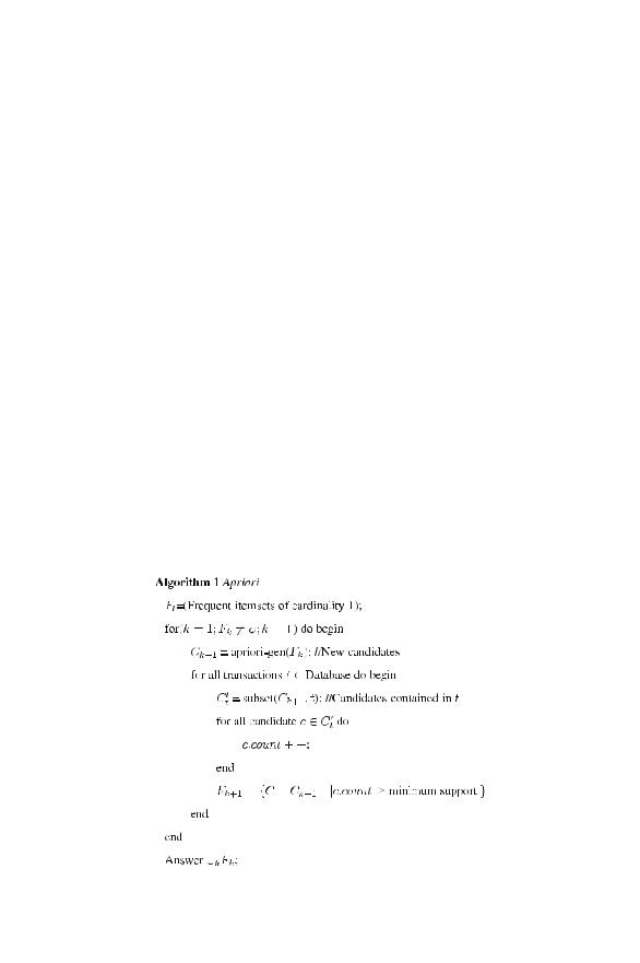
The Apriori algorithm is shown in Fig. 3. Function apriori-gen in line 3 generates Ck+1 from Fk in the following two step process:

1.Join step: Generate RK +1, the initial candidates of frequent itemsets of size k + 1 by taking the union of the two frequent itemsets of size k, Pk and Qk that have the first k − 1 elements in common.

2.Prune step: Check if all the itemsets of size k in Rk+1 are frequent and generate Ck+1 by removing those that do not pass this requirement from Rk+1. This is because any subset

of size k of Ck+1 that is not frequent cannot be a subset of a frequent itemset of size k + 1.

Function subset in line 5 finds all the candidates of the frequent itemsets included in transaction t. Apriori, then, calculates frequency only for those candidates generated this way by scanning the database.

It is evident that Apriori scans the database at most kmax+1 times when the maximum size of frequent itemsets is set at kmax.

The Apriori achieves good performance by reducing the size of candidate sets (Fig. 3). However, in situations with very many frequent itemsets, large itemsets, or very low minimum support, it still suffers from the cost of generating a huge number of candidate sets

Fig. 3 Apriori algorithm

123