matesha
.doc-
VfubSet of numbers:

-
Definition of function:

-
Intersection is
-
Union is A∪B
-
Disjoint is A∩B=ø
-
Sequence is bounded below if

-
Sequence
 is strictly decreasing if

-
Sequence
 is divergent if sequence
is oscillating or tending to infinity
is divergent if sequence
is oscillating or tending to infinity -
Bounded sequence

-
Definition of limit of sequence is

-
Sequence is monotone if

-
Monotone convergence principle If
 is an increasing sequence and bounded above, then it is convergent
sequence
is an increasing sequence and bounded above, then it is convergent
sequence -
Theorem of Bolzano-Weiertrasse: every bounded sequence of complex numbers has A convergent subsequence
-
Caushy sequence is Convergent, i.e. if given any ε>0, there exist N=N(ε)∈ℝ, depending on ε, such that
 whenever m>n≥N
 -
Composite function is
-
Inverse function for
 is
is 
-
Limit of function in since “ε-δ” is


-
 is
infinitesimal value
is
infinitesimal value -
 is infinitely
large value
is infinitely
large value -
Two Remarkable limits

-
 Function f(x) is continuous in point a
-
Point of discontinuity of first kind (common definition) There are the finite limits exist:
![]() ,
,
![]() ,
,
![]()
-
Points of discontinuity of second kind: If at least one limit
 does not exist or equals to ∞
 -
Points of discontinuity of first kind – jump point:

-
Points of removable discontinuity
 third condition is not satisfied
-
BOLZANO-WEIERSTRASS THEOREM 1 Suppose function y=f(x) continued on interval [a,b], so function y=f(x) is bounded on interval [a,b]
-
BOLZANO-WEIERSTRASS THEOREM 2 Suppose function y=f(x) continued on interval [a,b], so function y=f(x) reaches maximum and minimum on interval [a,b]
-
BOLZANO-CAUCHY THEOREM Suppose function y=f(x) continued on interval [a,b] and f(a)<0 and f(b)>0 or f(a)>0 and f(b)<0, so there exist such ξ∊(a,b): f(ξ)=0
-
Derivative of function f(x) in point x=a is

-
 ,
where v is speed, s is distance, t is time Physical
interpretation of derivative
,
where v is speed, s is distance, t is time Physical
interpretation of derivative -
Differentiation rules
-
Differentiation rules
-
Differentiation rules
-
Differentiation rules
-
If for
 the inverse function exists and
  ,
then
,
then -
Differentiation rules
-
Differentiation rules
-
Differentiation rules
-
Chain rule of differentiation

-
Derivative of n order Differential is main part of increment linearly with regard to 𝛥x: dy=f’(x)𝛥x
-
Form of differential dy (in contradistinction to derivative) Is invariable
-
L’hopital’s rule

-
A function f(x) is said to have stationary point at x=a if
-
A function f(x) is said to have a local maximum at x=a if
-
A function f(x) is said to have a local minimum at x=a if
-
If f’(x)>0 for every x<a in I and f’(x)<0 for every x>a in I, then
-
If f’(x)<0 for every x<a in I and f’(x)>0 for every x>a in I, then
-
Function f(x) is differentiable at every x∈I, and that f’(x)=0 and if f’’(x)<0, then
-
Function f(x) is differentiable at every x∈I, and that f’(x)=0
-
Function y=f(x) is concave upwards in interval [A,B], if for any x₁, x₂∈[A,b}

-
Function y=f(x) is concave down in interval [A,B], if for any x₁, x₂∈[A,b}

-
Inflection point is point of continued function dividing intervals of concavity (upwards and down)
-
Prerequisite of inflection point
-
Sufficient condition of inflection point: Recall (x₁, x₂, …, x𝓃) is critical point of function z and partial derivatives of second order exist and continued.
-
Asymptote of y=f(x) is
-
Let function y=f(x) is defined in ε of x₀ and lim f(x)=∞ as x→x₀-0 or lim f(x)=∞ as x→x₀+0
-
Antiderivative is function F(x) such that F’(x)=f(x)


-
Standard integrals
-
Standard integrals
-
Standard integrals
-
Standard integrals
-
Standard integrals
-
Integration by substitution: If we maks a substitution x=g(u), then dx=g’du
-
Integration by substitution
-
Integration by parts
-
Integration of irrationalities of kind
 can be rationalize by substitution
![]()
-
Integration of irrationalities of kind
 can be rationalize by substitution:

-
Integration of trigonometric functions
 can be rationalized by substitution

-
Integration of trigonometric functions
 can be rationalized by substitution
 -
Integration of trigonometric functions
 can be rationalized by substitution
 -
Integration of trigonometric function
 can be rationalized by substitution
 -
Non-integrable (in finite form) functions
-
Non-integrable (in finite form) functions:
-
Non-integrable (in finite form) functions:
-
Non-integrable (in finite form) functions:
-
Non-integrable (in finite form) functions:
-
Non-integrable (in finite form) functions:
-
Non-integrable (in finite form) functions:
-
By the definite integral


-
Newton-Leibniz Formulae: Suppose that a function F(x) satisfies F’(x)=f(x) for every x∈[A,B]. Then

-
Property of definite integralLinearity

-
Property of definite integral
Additivity:
![]()
-
Property of definite integral
Monotonness:
If f(x)≤g(x),
and a<b, then ![]()
-
Property of definite integral

![]()
-
Non-eigenvalue integral in half-interval [a,+∞)

-

If this limit exists and finite, then non-eigenvalue integral is convergent
If this limit does not exists or infinite, then non-eigenvalue integral is divergent
-
Particularly if non-eigenvalue integral
 is divergent, but
  exists, so
  is Value
Principal of
Integral
is Value
Principal of
Integral -
Multiplication of matrix

-
 Transpose matrix
-
Row echelon form of matrix is

-
Determinant of matrix 3x3 - Rule of triangles or Rule of Sarrus

-
Determinant of matrix 2x2 :A=


-
det(A)=0 singular
-
det(A)≠0 non-singular
-
This matrix
 Is augmented
-
An nxn matrix A is said to be invertible if if there exists an nxn matrix B=
 such that AB=BA=I
 -
Matrix I is Identity matrix if

-
Matrix with members
 is is
Identity matrix
is is
Identity matrix -
 ,
then multiplicative inverse is
,
then multiplicative inverse is

-
Minor is

-
Cofactor
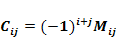 ,
where
,
where 

-
 where
K
is the adjoint of matrix A
where
K
is the adjoint of matrix A -
Trace of matrix is the sum of diagonal elements
-
Rank of a matrix is

-
Theorem of Kronecker-Capelli (Solution of system of linear equations)

System is inconsistent
System is consistent
-
Cramer’s Rule (solution of system of linear equation using matrix analysis). Suppose that the matrix A is invertible. Then the unique solution of the system Ax=b, where A, x and b are variables of system of linear equations where

-
Gaussian Elimination (Matrix Analysis)
![]()
The method of Gaussian Elimination reduces any set of linear equations to this triangular form by adding or subtracting suitable multiples of pairs of the equations.
-
A vector is an object which has magnitude and direction
-
For any vector u=(u₁, u₂) in ℝ², Norm of vector is real non-negative number

-
Scalar products of vectors

-
Economic interpretation of scalar products of vector
![]() -
summary value of goods
-
summary value of goods
where
![]() - vector of volume of different goods,
- vector of volume of different goods,![]() - vector of prices of different goods
- vector of prices of different goods
-
Orthogonality condition for vectors: cos θ = 0 (by θ=π⁄2) ⇒ u₁v₁+u₂v₂+u₃v₃=0
-
Colinearity condition for vectors v₁/u₁=v₂/u₂=v₃/u₃
-
Orthogonal projection of vector. Suppose that u, a∈ℝ³. Then

-
Scalar triple product of vector is

-
Perpendicular distance D of a plane ax+by+cx+d=0 from a point (x₀, y₀, z₀) is given by

-
Suppose that
 are vectors in a vector space V over R. By a linear combination of
the vectors
are vectors in a vector space V over R. By a linear combination of
the vectors  ,
we mean an
expression of the type
,
we mean an
expression of the type  ,
where
,
where  ∈ℝ
∈ℝ -
Suppose that
 are vectors in a vector space V over ℝ:
 are linearly dependent if
there exist
are linearly dependent if
there exist  ,
not all zero, such that
,
not all zero, such that 
-
Suppose that
 are vectors in a vector space V over ℝ:
 are linearly independent if
the only solution of
are linearly independent if
the only solution of  is given by
-
Suppose that
 are vectors in vector space V or R. We say that {
 is
a basis for V if the
followig two conditions are satisfied:
is
a basis for V if the
followig two conditions are satisfied:
a){![]() =V
=V
b)The
vectors ![]() are linearly independent.
are linearly independent.
-
Dimension dim(V) of vector space V is maximum number of linearly independent vectors
-
THEOREM of matrix of transformation . Matrixes A and A* of linear operator
 over basis (
 )
and basis ((
)
and basis (( )
can be coupled as:
)
can be coupled as:
 ,
where C
is matrix of transformation from old basis to new basis.
,
where C
is matrix of transformation from old basis to new basis.
-
DEFINITION. “Quadratic form “
 of n variables
 or
or  where every element is either squared variable, or scalar
multiplication of 2 different variables.
where every element is either squared variable, or scalar
multiplication of 2 different variables.
![]()
-
Eigenvalue is solution of characteristics equation

-
Quadratic form has canonical form, if

-
Elements of Analytical Geometry: Relationship between Polar and Cartesian Co-ordinates: Superimpose one diagram upon the other a) X=r cosθ and y=r sin θ
b)
![]() and
and ![]()
-
Elements of Analytical Geometry: A straight line is a set of points with cartesian co-ordinates (x,y) satisfying an equation of the form ax+by+c=0, where a, b and c are const.
-
Elements of Analytical Geometry: Equation of a line passing through 2 given points

-
Elements of Analytical Geometry: Distance between 2 points

-
First order differential equation y’=f(x,y) is called incomplete if it does not contain (obviously) or the function itself with, or independent variable x: y’=f(x) or variable y: y’=f(y).
-
The differential equation of the form y’=f(x)g(y) called a differential equation with multiple variables
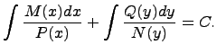
-
Linear differential equation of first order is an equation that is linear in the unknown function and its derivative, if

-
First-Order Homogeneous Equations:

-
Differential equation y’’+a₁y’+a₀y=f(x), where coefficients a₁, a₀ are const, linear differential equations of second order with fixed variables .
-
Differential equation y’’+a₁y’+a₀y=f(x) where coefficients a₁, a₀ are constants, called linear differential equations of second order with fixed variables. If f(x)=0, then this equation called non homogeneous
-
Differential equation y’’+a₁y’+a₀y=f(x) where coefficients a₁, a₀ are const, called called linear differential equations of second order with fixed variables If f(x)≠0, then this equation called homogeneous
-
Fundamental system of solutions
-
Functions y₁(x), y₂(x) called linear depended in interval (a,b) if there are exist constant numbers λ₁, λ₂ not equal to zero, such a λ₁y₁(x)+λ₂y₂(x)=0 for every x∈(a,b) . If this condition executes in a case when λ₁=0 and λ₂=0, so functions y₁(x), y₂(x) called linear independed in interval (a,b).
-
Solution of homogeneous linear differential equations of second order with fixed variables: y’’+a₁y’+a₂=0: characteristic equation( to change in a homogeneous equation derivatives from initial function to K in appropriate power)
 a₂=0
has 2 solution: k₁
and k₂,
then general solution is
a₂=0
has 2 solution: k₁
and k₂,
then general solution is 
-
Solution of homogeneous linear differential equations of second order with fixed variables: y’’+a₁y’+a₂=0: characteristic equation( to change in a homogeneous equation derivatives from initial function to K in appropriate power)
 a₂=0
has 1
solution: k₁=k₂=k,
then general solution is
a₂=0
has 1
solution: k₁=k₂=k,
then general solution is 
-
Solution of homogeneous linear differential equations of second order with fixed variables: y’’+a₁y’+a₂=0
-
Solution of non-homogeneous linear differential equations of second order with fixed variables: y’’+a₁y’+a₂=f(x):solution of system of equations
-
Caushy problem for differential equations: Caushy task – is a one of the main task in the theory of differential equations (ordinary and partial); it is consisted in
searching a solution (integral) of the differential equation, satisfying, so-called, initial conditions (initial data).
Let the function f(x) is a well defined value in D for . We should find a solution which satisfying initial conditions.
Caushy Task: If in D, function f (x, y) is continuous and has continuous partial derivatives , so for any pointin a neighborhood of corresponds only an unique solution
-
Common member of series
 :
Number
:
Number
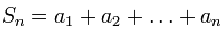 is sum of numerical series
 -
Sum of numerical series
 is
common
member of numerical series
is
common
member of numerical series -
Numerical series is convergent, if
 exists and finite, then

-
Numerical series is divergent, if (lim is not exists or =∞)
-
Property of convergence of numerical series

-
Property of convergence of numerical series

-
Property of convergence of numerical series:

-
Prerequisite of convergence of numerical series

-
Harmonic series is sum of infinite quantity of members reversed to serial natural numbers

-
Series is harmonic if because of each three members starting second
 satisfies
to one rule
satisfies
to one rule

-
Generalized harmonic series

-
THEOREM OF D’ALAMBER (for series) If for series with positive members

![]() is
valid, then the numerical series is convergent by l<1 and
divergent by l>1
is
valid, then the numerical series is convergent by l<1 and
divergent by l>1
-
THEOREM OF CAUSHY (for series) Let for positive defined series
 the limit exists
 then if l<1, series is convergent, if l>1, series is
divergent, if l=1, convergence question is open.
then if l<1, series is convergent, if l>1, series is
divergent, if l=1, convergence question is open. -
THEOREM OF LEIBNIZ (criteria of series convergence). Sign-alternative series
 is convergent if


-
Sign-variable series
 Its
members can be positive and negative
Its
members can be positive and negative -
THEOREM (sufficient condition of convergence for sign-variable series).

-
Series
 is absolute
convergent
is absolute
convergent
-
Series
 is conditional
convergent
is conditional
convergent
-
Consequence of Theorem of Leibniz Following Theorem of Leibniz we can evaluate error of sum calculation

-
Determine the domain of the function:
 =[1;+∞)
 -
Determine the domain of the function:
 x≠±2
x≠±2
-
Determine the domain of the function:
 =x>4
x≠7
=x>4
x≠7 -
Determine the domain of the function:
 x>1
x≠3
x>1
x≠3 -
Determine the domain of the function:
 (0;2)
(0;2) -
Find the limit of the function:
 =4
=4 -
Find the limit of the function:
 =10
=10 -
Find the limit of the function:
 =2/5
=2/5 -
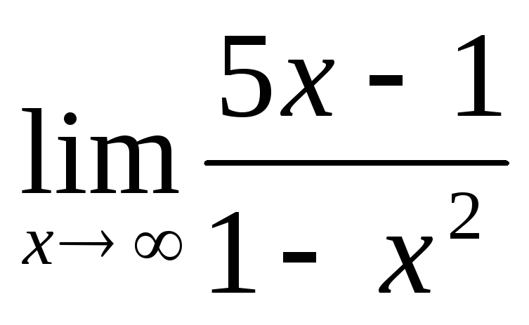
Find the limit of the function:
 =-1/2
=-1/2 -
Find the limit of the function:
 =3
=3 -
Find the limit of the function:
 =0
=0 -
Find the limit of the function:
 =5
=5 -
Find the limit of the function:
 =4
=4 -
Find the limit of the function:
 =8
=8 -
Take derivative of the function:
 =42xcos(7x^2-1)
 -
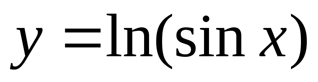
Take derivative of the function:
 =5/2*√(x+3)
 -
Take derivative of the function:
 =2xlnx+x
 -
Take derivative of the function:
 =ctgx
=ctgx -
Take derivative of the function:
 =-tgx
=-tgx -
Take second order derivative of the function:
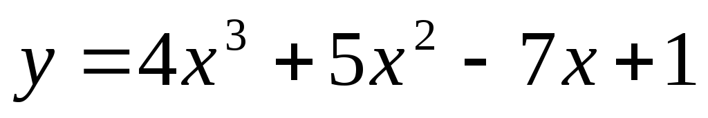 =24x+10
 -
Take second order derivative of the function: y = sinx=-sinx
-
Take derivative of the function: y = (sinx)3 =3(sinx)^2*cosx
-
Take derivative of the function: y = (lnx)2 =2lnx/x
-
Take derivative of the function: y =
 =1/2√x
 -
Take derivative of the function: y =
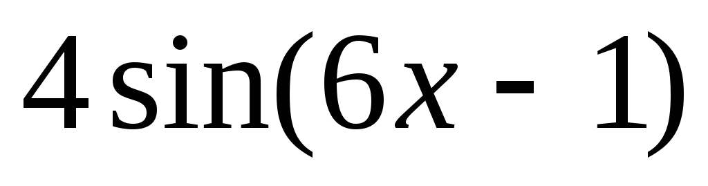 =24cos(6x-1)
 -
Take derivative of the function: y =
 =3*23x+2*ln2
 -
Take derivative of the function: y =
 =2*72x+5
*ln7
=2*72x+5
*ln7 -
Take derivative of the function: y =
 =3(5x^2
-4x +1)^2*(10x-4)
=3(5x^2
-4x +1)^2*(10x-4) -
Find the interval where the function is increasing:
 =(-∞;-3)
(1;+∞)
=(-∞;-3)
(1;+∞) -
Find the interval where the function is decreasing:
 (1;3)
(1;3) -
Find the extreme points of the function :
 =xmax=
3 xmin=1 o y(1)-max and y(3)
-min
=xmax=
3 xmin=1 o y(1)-max and y(3)
-min -
Find the extreme points of the function :
 xmax=4
xmin=2 y(2)-max and y(4) -min
xmax=4
xmin=2 y(2)-max and y(4) -min
-
Find the extreme points of the function :
 x=3
y=3
x=3
y=3 -
Find the interval where the function is concave up:
 (-1;+∞)
 -
Find the interval where the function is concave down:
 (-∞;-1)
 -
Find the points of inflection of the function:
 =-1
=-1 -
Find the interval where the function is concave up:
 =(2;+∞)
 -
Find the interval where the function is concave down:
 (-∞;2)
 -
Find the points of inflection of the function:
 =2
=2
-
Find the equations of the vertical asymptotes of the function:

-
x= -3 and x=3
-
Find the equations of the vertical asymptotes of the function:
 =x=
-5 and x=5
=x=
-5 and x=5 -
Find the equations of the horizontal asymptotes of the function:
 =Y=2
=Y=2 -
Find the equations of the horizontal asymptotes of the function:
 =Y=3
=Y=3 -
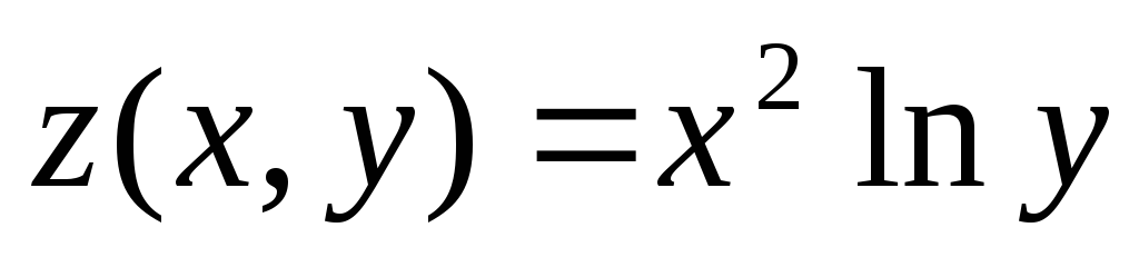
Find the partial derivative
 of
the function of two variables:
of
the function of two variables:
-
Find the partial derivative
 of
the function of two variables:
of
the function of two variables:
-
Find the partial derivative
 of
the function of two variables:
of
the function of two variables:
-
Find the partial derivative
 of
the function of two variables:
of
the function of two variables:
-
Find the partial derivative
 of
the function of two variables:
of
the function of two variables:
-
Find the partial derivative
 of
the function of two variables:
of
the function of two variables:
-
Find the partial derivative
 of
the function of two variables:
of
the function of two variables: