Advanced_Renderman_Book[torrents.ru]

Figure 2.10 A signal that is adequately sampled (top) and a signal that is inadequately sampled, which therefore aliases (bottom).

lost, but no low-frequency aliases are added in their place, and the image appears slightly blurry. Keep in mind, however, that supersampling only raises the bar-it does not entirely eliminate the problem. Frequencies even higher than the supersampling rate may still exist, and those will still alias even with the supersampling.

The second way around the conundrum is for our samples to be irregularly spaced, a technique known as stochastic sampling. Supersamples are still used, but the fact that they are not regularly spaced helps them weed out higherthan-representable frequencies in an interesting way. Using this technique, highfrequency data is still lost, but it is replaced by a constant low-intensity white noise that makes images look grainy. This is not better than abasing in a quantitative way, but due to certain perceptual tricks of the human visual system, this white noise is often a "less objectionable artifact" than the abasing. This process only works well when many supersamples are available to make up the final regularly spaced discrete pixel.

Once we have the required samples of the image "signal," the second critical phase of the antialiasing process is reconstructing the signal. In loose terms, this

2 Review of Mathematics and Computer Graphics Concepts

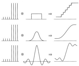
Figure 2.11 Several reconstruction filters operating on identical samples creating very different reconstructions of the signal.

is the process wherein the supersamples are averaged together to create the final pixels. The weights that are applied to each sample in the "weighted average" mentioned above come from the reconstruction filter. In less loose terms, reconstruction creates a new continous signal that we deem to be the best representation of the true signal that we can guess, given the point samples that we have. We pluck our output samples (the final pixels) from this reconstructed signal. Reconstruction proceeds by the convolution of the filter with the known supersamples. Different reconstruction filters give different results (see Figure 2.11), introducing new artifacts into our image that we know as blurring (when sharp edges become visible ramps in the output) and ringing (when sharp edges create waviness in the output).

Actually, there is a third way to reduce aliasing, which is to construct the scene so that the high-frequency data never exists in the first place and therefore never needs to be removed. This technique is known as prefiltering the scene and is a quite useful technique in situations where the signal is constructed from functions of other signals, such as is described in Chapter 11.

It would be a mistake to think that renderers are only worried about the spatial, or geometric, aliasing that causes "jaggies." Abasing can and does occur in any rendering process where sampling takes place. For example, rendering a moving scene at a moment in time causes temporal aliasing. Rendering by representing color spectra by only the three RGB color samples can cause color aliasing. Aliasing happens in a wide variety of dimensions, and the techniques for reducing or ameliorating the effects of aliasing are similar in all of them.

2.4 Computer Graphics

2.4.2Quantization and Gamma

The physical equations of light transport, and the approximations that are used in computer graphics, compute light intensity and color values with real numbers. However, most output devices are controlled by integer pixel values. The process of converting the floating-point real values into integers is called quantization. There are three special details that must be taken into account during quantization-bitdepth, gamma correction, and dithering.

Quantization converts the floating-point intensity values into the appropriate integer values for the output display based on their bit-depth. Devices vary in their ability to re-create subtle differences in color. For example, most computer monitors have the ability to reproduce only 256 different color levels (per color component or channel), whereas film is much more sensitive and can reproduce several thousand color levels. As a result, images that are computed for display on standard monitors will typically be converted to 8 bits per channel, whereas images computed for film may be converted to 10 to 14 bits per channel. The original floating-point numbers are scaled so as to convert 1.0, which requests the maximum intensity that the output device can attain, into the integer pixel value that will attain that intensity

All physical display media, be they film, hard-copy prints, or computer monitors, have a nonlinear response to input intensity. Small increments in pixel values in the dark regions create a smaller change in output intensity than the same increments in pixel values in the lighter regions. One effect of this is that when a device is given a pixel value of 0.5, the visual result the device produces will not appear to be intensity 0.5, but actually something less. For this reason, when integer pixel values are displayed on the device, they are often gamma corrected. This means that the dark values are pumped up along a curve like the one shown in Figure 2.12 to compensate for the device's laggardness. This curve is generated by the function out = inlly, where y (gamma) is a constant chosen appropriately for the display. Typical computer monitors, for example, will have a gamma between 1.8 and 2.4. Gamma correction restores the linearity of the image, so that linear changes in the computed light intensity will result in linear changes in the device's emitted image intensity.

A side effect of the nonlinear response is that output devices have more available pixel values in the darks (that is, more than half of the input values will create output intensities less than 0.5). However, passing the pixel data through a gamma curve upon display will skip over a lot of these values, and we can often see the multilevel jumps. To compensate for this, some images will be stored with a few more bits per channel, so that there is some extra precision for use in the darks, or with gamma correction already applied to the pixel values, or in a logarithmic format like Kodak's Cineon, which concentrates its available pixel values at the low end.

However, it is important to notice that the appropriate y is a function of the device that the image is being shown on, and the image needs to be recorrected if it

2 Review of Mathematics and Computer Graphics Concepts

42

Figure 2.12 A typical gamma curve, with y = 2.2.

is shown on a different device. Moreover, the standard image processing calculations that might be applied to an image, such as blurring, resizing, or compositing, all work best if the data is "linear," that is, has no built-in gamma correction. For this reason, it is usually best for high-quality images to be stored with no gamma correction and to apply correction as the image is being loaded into a display.

There are three ways to convert the floating-point intensity values to integers: truncation, rounding, and dithering. Truncation is the easiest, just use the floor function to drop the fractional bits after scaling. However, it is easy to see that this will drop the overall intensity of the entire image by a tiny amount, so perhaps rounding is better. Rounding means use floor if the fraction is less than 0.5 and cei 1 i ng if the fraction is more than 0.5. However, even rounding has an unfortunate effect on the appearance of the image because areas where the floating-point pixels are nearly identical will form a large constant-colored block once quantized. At the edge of this region, the color will abruptly change by one pixel level, and there will be the appearance of color "stair-stepping" in a region that should be a continuous gradient. These effects can be eliminated by dithering.

The term dithering is used confusingly in computer graphics to mean several different algorithms that have one thing in common: raising and lowering pixel values in a constant-colored region to simulate more bit-depth in a device that has too few output levels. Halftone dither and ordered dither describe algorithms that trade off spatial resolution to get more apparent color depth in a device that has lots of resolution but very few color levels. That's not the kind of dither we are referring

to. Quantization dither is a tiny random value added to floating-point pixel values just before they are truncated to integers. In a sense, it randomizes the choice between using floor and cei 1 i ng to do the conversion. This has the effect of breaking up these constant-colored blocks, making them less regular and almost fuzzy, so that on average the pixels in the region have the intended floating-point intensity. Another algorithm that accomplishes the same goal is error-diffusion dither, which computes the difference between the floating-point and integer versions of the image and makes sure that all of the image intensity is accounted for.

2.4.3Mach Bands

The human eye is extremely sensitive to boundaries and edges. Our vision accentuates these boundaries-a perceptual trick that makes them more noticeable. In fact, any time dark and light areas abut, our vision perceives the dark area getting even darker near the boundary and the light area getting even lighter near its side of the boundary, so as to enhance the contrast between the abutting colors. This effect is often so strong that we actually appear to see bands outlining the edge several shades off from the true color of the region. These bands are called Mach bands, after the psychophysicist Ernst Mach who first studied them in the late nineteenth century. 2

Unfortunately for computer graphics images, boundaries between large regions of constant or slowly changing colors are common, and the resulting Mach bands are noticeable artifacts (even though they aren't really there!). Mach bands are also visible when the slope of a color ramp changes suddenly along an edge; in other words, if there is a boundary in the derivative of the color. These effects are illustrated in Figure 2.13. In the figure, the graph below each image shows the actual and perceptual pixel values in the image. Notice that in the image on the right there is no discontinuity in the actual pixel values across the edge. The appearance of the lighter strip in the center is entirely perceptual.

2.4.4Coordinate System Handedness

Three-dimensional coordinate systems come in two varieties, known as left-handed and right-handed. The difference between these varieties is based on the directions that the coordinate axes point relative to one another. For example, if the x-coordinate axis points right, and the y-coordinate axis points up, then there are two possibilities for orienting the z-coordinate axis: towards the viewer or away from the viewer. Hold one of your hands up, with thumb and forefinger extended

2 This is the same Mach who defined the concept of Mach number for objects moving faster than the speed of sound.

2 Review of Mathematics and Computer Graphics Concepts

44

Figure 2.13 A Mach band between two constant-colored regions (left) and a Mach band delineating the change in color ramp slope (right). The graphs under the images illustrate the actual pixel values and the apparent pixel values.

like a capital L. The thumb points right along x, and the forefinger points up along y. If the z-axis points away from the viewer, this is termed "left-handed", because if you use your left hand, you can (somewhat uncomfortably) extend your middle finger (yes, that one) away from the viewer along the z-axis. If the z-axis points towards the viewer, this is termed "right-handed," because you need to use your right hand to extend your middle finger toward the viewer. Don't just sit there readingtry it! The physics students in the room perhaps recall a slightly different set of dexterous digit machinations from studying electromagnetic fields, where you hold your hand flat, fingers and thumb outstretched. With palm up, point your fingers right along x. You can then bend (curl) them to point up along y (we often say "rotate x into y"). The thumb then points along z. Same-handedness result: left hand gives you z away from the viewer, right hand gives you z toward the viewer.

Transformations that change the handedness of a coordinate system are called mirror transformations. Scaling by a negative value on one (or three) axes does this, as does exchanging any two axes.

Now we can answer the most probing question in all of human history. Why do mirrors reflect left-right, but not top-bottom? You can turn sideways, spin the mirror, stand on your head, but it always does it. Is this because we have two eyes that are next to each other left-right? (No,obviously not, because it happens even if one eye is closed . . . .) Does it have something to do with the way our brains are wired, because we stand vertically, so our eyes are immune to top-bottom swaps? (No, it can't be simply perceptual, because we can touch our reflection and everything matches . . . .)

The answer is, a mirror doesn't reflect left-right. Point down the positive x-axis (right). Your mirror image also points down the positive x-axis. Right is still right.

Left is still left. Up is still up, down is still down. What is swapped is front-back! Our nose points away from the viewer (positive z), but the reflection's nose points toward the viewer (negative z). If it didn't swap

front-back, we'd see the back of our heads. And guess what, the sole axis that is swapped, the z-axis, is the one that is perpendicular to the plane of the mirror-the one axis that doesn't change if you spin the mirror or yourself.

2.4.5 Noise

In his 1985 Siggraph paper, Perlin developed the concept that is commonly known today as noise. Image and signal processing theory, of course, had already studied many different types of noise, each with a name that indicated its frequency content (e.g., white noise, pink noise). But signal processing noises all share one important quality: they are intrinsically random. Perlin recognized that in computer graphics, we want functions that are repeatable, and thus pseudorandom. But even more, he discovered that we get more utility out of functions that are random at a selected scale but are predictable and even locally smooth if seen at a much finer resolution.

The noise functions that Perlin developed, and the ones that were later developed by other researchers, all have similar properties:

•deterministic (repeatable) function of one or more inputs

•roughly bandlimited (no frequency content higher than a chosen frequency)

•visually random when viewed at scales larger than the chosen frequency

•continuous and smooth when viewed at scales finer than the chosen frequency

•having a well-bounded range

These properties give Perlin noise two important capabilities when used in computer graphics-it can be antialiased and it can be combined in a manner similar to spectral synthesis. Antialiasing comes from the fact that noise has controlled frequency content, which makes it possible to procedurally exclude frequencies that would lead to abasing later in the rendering process. Spectral synthesis is the technique of layering different frequencies at different intensities to create complex and interesting patterns. Many natural patterns have a similar kind of controlled random appearance, random over a set of frequencies but controlled at higher and lower ones. Perlin noise provides an interesting tool to simulate these and other patterns.

2.4.6 Compositing and Alpha

It is usually the case in image synthesis that the final image is made up of a combination of several images that each contain part of the data. For example, the image might be computed in layers, with the objects close to the camera rendered in one image and the images in the background rendered separately. In conventional special effects photography, optically combining the images is known as matting or composite photography and is done on a device called an optical printer. However,

46 2 Review of Mathematics and Computer Graphics Concepts

only three operations are available on an optical printer: adjusting the exposure or focus of an image, multiplying two images together (often used to cut a piece out of an image), and multiple exposure (adding two images together). Creating a multilayered effect requires multiple passes through the optical printer, with generation loss at each step.

Compositing of digital images, however, can do anything that can be programmed, to any number of images, and with no generation loss. The most common operation is layering two images on top of one another, with the "background" image showing through only where the "foreground" image is vacant-an operation called over. Determining where the image actually has data and where it is vacant is tricky for live-action footage and involves various combinations of rotoscoped mattes and blue/green-screen extraction, but for computer-generated footage it is quite easy. The renderer tells you, by storing this information in a separate image channel called the alpha (a) channel. In 1984, Porter and Duff described an algebra for combining images using the a channel of each image.

Modern paint packages often include the concept of mattes and matte channels, but a is a very specific version. First, painted mattes are often one bit deep, identifying if the pixel is in or out. In order to be useful in a world where synthetic pixels are well antialiased, the a channel usually has as many bits as the other color channels. Second, painted mattes with multiple bits (known as fuzzy mattes) are stored without modifying the actual color data. Extracting the intended image requires the program to multiply the color by the matte, using all of the image color where the matte is full-on, a fraction of the color in the fuzzy regions, and black where the matte is full-off. a, on the other hand, is stored premultiplied into the color channels. In places where the matte is full-on, the color channels hold the full-intensity color. In the fuzzy regions, the color channels themselves are predimmed. Where the matte is full-off, the color channels hold black. There are various advantanges in the rendering and compositing process that make this premultiplication scheme superior for encoding computer-generated images.

Digital images are now commonly stored in four channels-red, green, blue, and alpha, or RGBA. Of course, just having a fourth A channel does not guarantee that it contains a, as some software might store a matte value in the channel instead. In some sources, premultiplied alpha is called associated alpha, to distinguish it from matte data or other arbitrary data that might be stored in the fourth channel of an image.

2.4.7Color Mode

As mentioned in the previous section, light is a continuous phenomenon that can be accurately represented only as a complete spectrum. Color, on the other hand, is a psychophysical concept, because it refers to the way that we perceive light. Over the years, practitioners in the disparate fields of colorimetry, physiology, electrical engineering, computer graphics, and art have developed a variety of ways of representing color. With rare exceptions, these representations each have three

numeric values. The human eye has three kinds of color sensors, the cones. Any light presented to the cones stimulates them each by some amount depending on their sensitivity to the frequency spectrum of that light. This acts to "convert" the continuous spectral representation of the light into three independent samples, socalled tristimulus values, that we perceive as the color of the light. Because we perceive light in this three-dimensional color space, it is perhaps not surprising that most other color spaces also require three dimensions to span the full range of visual colors.

Interestingly, though perhaps also not surprisingly, there are many subtleties in the psychophysical study of color perception. For example, there are often many different light spectra that will stimulate our cones with the same intensity, and so therefore are the same color perceptually. These colors are called metamers, and without them, it would be impossible to re-create the appearance of color on a television display. Televisions (and computer monitors and laser displays, etc.) generate color using three guns with very specific (and sometimes very narrow) spectral output characteristics. These are made to look like a wide variety of colors because they create metamers for each light spectrum that the display needs to represent.

The most common representation of color in computer graphics is RGB: red, green, blue. This color scheme is simply the direct control of the colored guns of the television or computer monitor. The color channels range from 0.0, meaning the gun is off, to 1.0, meaning the gun is at maximum intensity. There are many other color models that are piecewise linear transformations of the RGB color model. Some of these color models, such as HSL (hue, saturation, lightness) and HSV (hue, saturation, value), were created because the triples were more intuitive to artists than the RGB tristimulus values. Other models, such as the television color models Y'IQ (which obviously stands for luminance, in-phase, and quadrature) and Y'UV, were created because they model a specific color output device or an analog signal encoding. In each case, a simple linear equation or simple procedure converts any value in one color model to a value in the other color models.

Notice, however, that these models don't specify exact colors. They merely describe the intensity of the guns (or other color generators) of the output device. If the guns on one device generate a different "base color" than the guns on another device (a relatively common occurrence, actually), then the resulting colors will appear different on the two devices. There are some color models that attempt to solve this problem by tying specific color-model values to specific light spectra. For example, the CIE is an international standards organization whose purpose is to quantify color, and they have created several specific color models that lock down colors exactly. The most widely used of these is CIE XYZ 1931. NTSC

RGB 1953 attempted to solve the same problem for television by specifying the exact CIE values of the "standard phosphors."3

3 Unfortunately, as technologies changed, these values quickly became obsolete.

2 Review of Mathematics and Computer Graphics Concepts

48

Printing processes, which need color primaries in a subtractive color space, often specify ink or die colors in the CMY (cyan, magenta, yellow) color model. Descriptions of CMY often appeal to the idea that cyan is the "absence of red," and therefore CMY = (1,1,1) - RGB. In fact, printing is a much too subtle process to be captured by such a simplistic formula, and good transformations of RGB to CMY (or to the related CYMK color model, which is CMY augmented by a channel of black ink) are proprietary trade secrets of printing companies.

Other color models solve a different problem. Because the human eye is more sensitive to color changes in some parts of the spectrum than others, most color models do not have the property that a constant-sized change in the value of one channel has a constant-sized apparent change in the color. Models that take these nonlinearities of color perception into account are called perceptual color spaces. Artists appreciate these models, such as the Munsell color model, because it makes it easier to create visually smooth gradations and transitions in color. CIE L*u*v* and CIE L*a*b* try to perform the same function in a mathematically more rigorous way with nonlinear transformations of standard CIE coordinates. Recently, image compression engineers have started to study these models because they help determine which are the "important bits" to save and which bits won't ever be noticed by the audience anyway.

The gamut of a device refers to the range of colors that it can reproduce. For example, there are many colors displayable on a computer monitor that ink on paper cannot reproduce. We say that ink has a "smaller gamut" than monitors. Figure 2.14 shows the relationship between the gamuts of NTSC RGB and a typical dye sublimation printer. Anyone who is trying to faithfully reproduce an image from one medium in another medium needs to be aware of the limitations of the gamuts of the two media and have a strategy for approximating colors that are outside of the new color gamut.

2.4.8Hierarchical Geometric Models

When we are building geometric models of complicated objects, it is often the case that one part of the model is connected to another part through some type of joint or other mechanism. For example, the shoulder, elbow, and wrist connect rigid body sections with joints that limit motion to particular rotations. This leads to hierarchical motion of the body parts, where rotating the shoulder joint causes the whole arm and hand to move in unison, whereas rotating the elbow causes only the lower arm and hand to move, and rotating the wrist moves only the hand. Each body part's position is always relative to the positions of the higher body parts.

Rather than model each body part separately, and make complex calculations to refigure the position of the hand every time any of the arm joints move, it is significantly simpler to encode the model's motion hierarchy directly into a treestructured hierarchical geometric model. Each body part lives at a node in the hierarchy, and the transformation stored at the node is relative to the immedi