Добавил:

Upload Опубликованный материал нарушает ваши авторские права? Сообщите нам.

Вуз:

Томский Политехнический Университет

Предмет:

[НЕСОРТИРОВАННОЕ]

Файл:

Buzug_Computed_tomography_From_photon_stat.pdf

Скачиваний:

Добавлен:

29.05.2015

Размер:

15.29 Mб

Скачать

☆

<<< < Предыдущая 1 2 34 / 74 5 6 7 > Следующая >>>

7Technical Implementation

Contents

7.1 Introduction . . . . . . . . . . . . . . . . . . . . . . . . . . . . . . . . . . . . . . . . . . . . . . . . . . . . . . . 241 7.2 Reconstruction with Real Signals . . . . . . . . . . . . . . . . . . . . . . . . . . . . . . . . . . . . . . . . 242

7.3 Practical Implementation of the Filtered Backprojection . . . . . . . . . . . . . . . . . . . . . . . 255

7.4 Minimum Number of Detector Elements . . . . . . . . . . . . . . . . . . . . . . . . . . . . . . . . . . 258 7.5 Minimum Number of Projections . . . . . . . . . . . . . . . . . . . . . . . . . . . . . . . . . . . . . . . . 259 7.6 Geometry of the Fan-Beam System . . . . . . . . . . . . . . . . . . . . . . . . . . . . . . . . . . . . . . . 261

7.7 Image Reconstruction for Fan-Beam Geometry . . . . . . . . . . . . . . . . . . . . . . . . . . . . . . 262 7.8 Quarter-Detector O set and Sampling Theorem . . . . . . . . . . . . . . . . . . . . . . . . . . . . . 293

7.1 Introduction

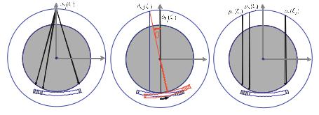
The geometrical design of a CT scanner is relatively simple. As already described in the preliminary remarks on CT in Sects. . to . , the development stages can be divided into four generations. Two of these generations – the ﬁrst and the third one – are particularly interesting. The ﬁrst generation – the pencil-beam concept – exactly reﬂects the Radon reconstruction process, since parallel beams deﬁne the slice plane (cf. Fig. . , middle and right side). The second generation is just a temporary intermediate developmental step toward the third generation, the fan-beam concept. The third-generation scanners (Fig. . , left side) are those most frequently implemented to date. For this reason, the focus of this chapter will be on the reconstruction mathematics based on fan-beam geometry.

The fourth generation is again a stage of evolutionary progress that has not yet been frequently implemented. From a mathematical point of view, this generation is identical to the third generation and will therefore not be considered here separately. The fast backprojection methods will not be considered here either. A good summary on modern reconstruction methods is given in Ingerhed ( ).

7 Technical Implementation

Fig. . . The currently most frequently used third-generation scanner (left) compared with the ﬁrst generation (center and right)

7.2

Reconstruction with Real Signals

The spectral weighting function, q , has the unit of a spatial frequency and is deﬁned for all frequencies, so that one has to integrate

	(		) =	+	(		)
	(		) =	−	(		)
hγ		ξ		∫ Pγ		q		q	e πiq ξ dq	( . )

along the whole frequency domain. As the real signal is spatially discrete and also spatially limited due to the limited number of detectors, the spectrum of the projection is repeated periodically as a result of the sampling process. In Sect. . it was reported that Shannon’s sampling theorem ensures faultless sampling of a signal with a sampling frequency, ξ = ( Q)− , if the maximum available spatial frequency is less than Q. Due to this, weighting of the periodic spectrum with the ramp function, q , is only reasonable in the interval [−Q, Q]. Let the sampled projection signal be

pγ (j ξ) , with j = , , . . . , D − .

( . )

The sampling parameters ξ (width of one single detector element) and D (number of the detector elements) can be easily changed in CT systems of the ﬁrst generation by means of tube and detector feeds. In systems of the third generation, which have been most frequently used to date, ξ is actually determined by the ﬁxed detector width and D by the ﬁxed number of detector elements. In this chapter it will be shown later on (cf. Sect. . ) that the sampling intervals can be synthetically halved by taking structural measures, such as a quarter detector shift or ﬂying focus concept.

In principle, the Fourier transform of the projection

Pγ (q) =	D ξ
Pγ (q) =	∫ pγ (ξ)e− πiq ξ dξ	( . )

7.2 Reconstruction with Real Signals

must now of course only be performed over the total detector length, i.e., over the interval [ , D ξ]. Outside the detector the projection is assumed to be zero. Pγ (q) can now be discretized by

D−

Pγ

pγ

e− πi(jk

D) ,

( . )

j =

where

and

Pγ (k

q),

with k = , , . . ., D −

( . )

q =

( . )

For the windowed high-pass ﬁltered projection

hγ(ξ)

−∫Q

Pγ (q) q e πiq ξ dq ,

( . )

the Fourier transform must be approximated. Obviously, only an approximation can be calculated because, from a mathematical point of view, the Fourier transform cannot be limited to [−Q, Q] (cf. Chap. ). This is due to the fact that the projection signal is in any case limited in the spatial domain by the ﬁnite length of the detector, as already described above.

However, the energy, which is physically contained in the high-frequency bands, can be neglected for a su ciently high value of D, i.e., a su ciently long detector array. Thus, a band limitation that is required to ensure a su cient sampling process, only destroys a small amount of information such that discretization can be expressed as shown:

(

)

Q D −

e πi(jk D) .

hγ

j ξ

k −D

Pγ

( . )

This equation yields the ﬁltered projection, hγ

ξ , at the sampling points, j ξ,

of the projection, p

ξ , by the inverse ﬁnite

and discrete Fourier transform of the

(

)

product of

and P

k Q D

in the frequency domain. The image to be

k Q D (

)

reconstructed

ﬁnally results from the discrete approximation of the integral

(

)

f (x, y) =

∫ hγ(ξ)dγ

( . )

(

) +

(

))

hγn

γn

y sin

γn

Np n =

x cos

7 Technical Implementation
where γn for n			, , . . ., Np are the angles of the measured projections since the
projection	angles are also just available as discrete values. The standardization in
projection		=
front of the sum in ( . ) is accomplished by the discretization of the angle element
			dγ	γ =	π
						.	( . )
					Np	.	( . )

In practice, it does not seem to be useful to multiply the frequency domain for real data with a linearly increasing function, as shown in ( . ), since linear spectral weighting increases the noise in the high frequency band. Therefore, the reconstructed tomogram may ﬁnally be degraded by unacceptably noisy signals. This can be remedied by means of suitable data windowing.

7.2.1

Frequency Domain Windowing

The Fourier transform theory lists a multitude of frequency or spectral windows. These are superior to a sharp rectangular band limitation within the frequency interval [−Q, Q] by means of the linearly increasing function given in ( . ).

Taking into account the window function in the frequency domain leads to the following approximation:

hγ j Q = hγ(j ξ)		D
		Q

D −

k=−D

Pγ k Q ?k Q ? W k Q e πi(jk D), D D D

( . )

where W is the corresponding window function. By the way, it makes no di erence whether the sum in ( . ) runs from −D to D − or from to D, since the sampled signals are part of a periodic spectrum (cf. Sect. . ).

There are several proposals concerning the shape of the window function. From these, a selection of eight are brieﬂy discussed, one by one, in the following paragraphs.

	Taking into account the linear weighting of the whole spatial frequency domain,
	G q	q for all q ,			( . )
this (theoretically) means no windowing;( ) = thus, W q					for all q. Ramachandran
and Lakshminarayanan ( ) have proposed to cut(			the frequency band with a rect-
and Lakshminarayanan ( ) have proposed to cut(				)
angle.
	The rectangle
or	W(q) = rect(q) ,				( . )
	G(q) = q rect(q)				( . )

7.2 Reconstruction with Real Signals

is in this case deﬁned by a normalized interval q = [−ε, ε] with ε = . , just to give one example. This approach is above all used to prevent weighting with q resulting in an excessively high noise increase in the high bands. In principle, the rectangular window must determine a unique interval for the periodic, discrete frequency band.

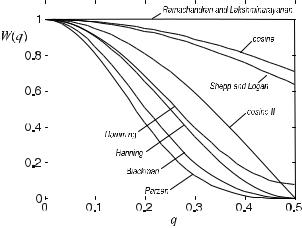
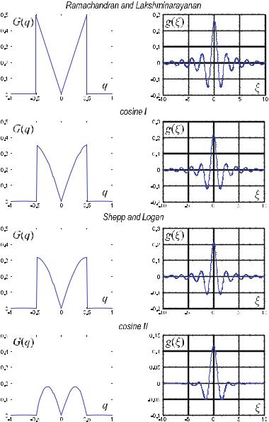
However, the sharp edges result in undesired sidelobes; thus, it seems to be useful to ﬂatten the edges of the window intervals. This provides a certain degree of freedom, which is used in CT to implement a variety of windows ranging from kernels that emphasize edges to ones that yield rather smooth images.

In order to prevent an excessively sharp window edge, a cosine function (cosine I in Fig. . ) is applied at ﬁrst to the rectangle, the argument of which ranges from −π to π , i.e.,

or	W(q) = rect(q)cos(πq )	( . )
	G(q) = q rect(q)cos(πq ) .	( . )

Shepp and Logan ( ) have made a similar proposal, which is most commonly used today

or	W(q) = rect(q)sinc(q)	( . )
	G(q) = q rect(q)sinc(q) .	( . )

The application of the sinc function to the rectangle proposed by Shepp and Logan yields a slightly smoother convolution kernel than that of cosine I in ( . ). However, as mentioned above, a multitude of windowing methods are described in the literature (Oppenheim and Schafer ) that are mainly aimed at making the window edge even smoother to prevent the formation of sidelobes with high energy in the convolution kernel. This may, for example, again be achieved by means of a cosine window; the argument of which ranges from −π up to π

or	W(q) = rect(q)cos(πq)	( . )
	G(q) = q rect(q)cos(πq) .	( . )

Here, attenuation in the frequency domain occurs without discontinuity such that the ripple content of the kernel can be better suppressed than with the abovementioned functions. For many applications in which sharp edges in the spatial domain are not such a decisive factor, even smoother kernels are used. In this context the following window functions of Hamming, Hanning, and Blackman, respectively, should be mentioned. All of these are based on the rectangle function to

7 Technical Implementation

which a properly selected term is added, consisting of a section of a cosine function with appropriate frequency and weighting factor. In fact, the spectrum of the cosine function partly compensates for the ripple content of the spectrum of the

rectangle function.
	The commonly referred to Hamming window is generated symmetrically
around zero with the interval q = [−ε, ε] where ε = .
or	W(q) = rect(q)( . − . cos( πq))									( . )
	G q	q rect q	.	. cos πq .
Accordingly, what is called( ) = the Hanning( )( window−					is generated( ))by					( . )
or	W(q) = rect(q)( . − . cos( πq))									( . )
	G q	q rect q	.	. cos		(	πq	))	,
and what is known as the( )Blackman= (window)( −by						(		))		( . )
or	W(q) = rect(q)( . − . cos( πq) + . cos( πq))									( . )
	G(q) = q rect(q)( . − . cos( πq) + . cos( πq)) .									( . )

Huesman et al. ( ) describe further windows with considerable attenuation of the higher frequencies, such as the Parzen window, which is listed below as a ﬁnal example.

rect(q) −

( −

)

(

-rect

) = /

( ) ( − )

or, respectively,

rect(q) q−

(

−

)

(

- rect q

q q

) = /

( ) ( − )

for q ε for ε < q ε

for q ε

for ε < q ε .

( . )

Figure . illustrates the di erent window functions given in the frequency domain.

	7.2 Reconstruction with Real Signals

Fig. . . Window functions used for band limitation by weighting the spectrum linearly

7.2.2

Convolution in the Spatial Domain

For many window functions, the kernels can be explicitly expressed in the spatial domain. As already described in Sect. . , the ﬁltering process in the frequency domain can equivalently be described in the spatial domain by a convolution. The convolution for continuous signals reads

(

)

(

−

)

hγ

∫ pγ

dz .

( . )

) =−

In Sect. . the di culties related to the integration of the Fourier integral with

non-square integrable functions have already been pointed out. The function

πξ

lim g

lim

( . )

β(

) =

− ( πξ )

= −

πξ

g(ξ) = β

must be considered as a distribution with a positive δ-peak at ξ

. However, this

(

+ (

) )

(

)

limit consideration is not really useful in practice.

In this special case, the situation is di erent since in real systems band-limited signals have to always be considered such that the linear weighting function, which is of relevance in practice, reads

G(q) = q rect(q) . ( . )

This weighting function has been deﬁned above as an example on the normalized interval q = [−ε, ε] with ε = . . The band limitation describes the regularization of the reconstruction problem introduced in Sect. . . , by means of which the

7 Technical Implementation

high frequencies are cut o . The regularization results in a su ciently smooth ﬁlter in the spatial domain for which a closed formula is available that can be explicitly calculated.

The regularized, i.e., band-limited kernel in the spatial domain will only be calculated in detail as an example of the windowing process for the cut-o described by Ramachandran and Lakshminarayanan. For this purpose, the inverse Fourier transform,

g(ξ) =	+ε	q ei π ξq dq = −		q ei π ξq dq +	+ε
g(ξ) =	−∫ε	q ei π ξq dq = −	−∫ε	q ei π ξq dq +	∫ q ei π ξq dq ,	( . )

of the ramp that is windowed by a symmetrical rectangle with a length of ε is calculated. The error, which arises from the fact that the high frequencies will be cut o , will then be negligible, if the frequency band of Pγ (q) is actually limited to the interval q = [−ε, ε]. This is often the case for real signals, since the projection represents an averaging process and thus acts as a low-pass ﬁlter. On simple radiographs, the poor image contrast is actually due to this averaging process.

Integral ( . ) is carried out via integration by parts, thus

∫ q eaq dq

eaq

∫

eaq

− eaq

( . )

= q

−

+ C =

a−

+ C

so that the result for ( . ) is

g(ξ) = −

πiξ−

( . )

e πiξq −ε +

e π i ξq .

πiξq

If the limits are

substituted, the above equation reads

)

(

−

)

−

(

−

( . )

(

) = −

−

πiξε

e− πiξε

πiξε

−

e πiξε

(

πiξ

)

(

πiξ

)

(

πiξ

)

(

πiξ

)

An evaluation of the bracketed expressions yields

g(ξ) =

−

e− πiξε

−

e− πiξε

e πiξε

πiξ

(

πiξ

( . )

(

)

e πiξε

)

πiξ

−

After sorting these(

expressions

(

)

− (

)

+ (

)

( .

( ) =

−

− (

g ξ

πiξ

e πiξε

πiξ

e− πiξε

πiξ

e πiξε

πiξ

e− πiξε ,

)

7.2 Reconstruction with Real Signals

the following sine or sinc expressions can be found in the above equation:

e πiξε

e− πiξε

eπiξε

e−πiξε

πξ

( ) =

−

sin πξε

sin

πξε

) −

πξε

(

ξε

( )

sinc

ξε .

With ε

this results in

) −

(

)

(

)

(

sin

( ) = * ,π ξ

(

) −

( ξ

and with the double angle formula for the cosine

this can be changed to

cos( x) = − sin (x) ,

sin (x) =

( − cos( x)) ,

( . )

which ﬁnally gives

sin

cos

! .

g ξ

( . )

*π

)

, −

( ) =

(

)

(

ξ ,

In analogy to the previous calculation, the kernel of Shepp and#Logan can be calcu-

lated by

(

) = −

−

ξsin *π

( . )

π ξ

−

(this result was given by Morneburg [ ]). Expressions for the Hanning and Hamming windows are listed by Huesman et al. ( ). As a ﬁnal example, the kernel of the Parzen window should be mentioned.

cos

sin π

cos

ξ ξ,

(

) =

* ξ , −

sin*

−

π,ξ

(

ξ)

( . )

ξ , − * ξ , −

Figure . shows the corresponding band-limited ﬁlter in the frequency and spatial domains respectively for the prominent windowing functions discussed above.

	7 Technical Implementation

Fig. . . Band-limited window functions of the ﬁltered backprojection in the frequency domain (always left-hand side) with the corresponding Fourier transforms in the spatial domain, i.e., the corresponding convolution kernels (always right-hand side). The sampling interval is set to ξ =

		7.2 Reconstruction with Real Signals

Fig. . . Band-limited window functions of the ﬁltered backprojection (continued)

The common aspect of the di erent windowing functions is that even spatial frequencies below the maximum interesting frequency are attenuated. For this reason, the spatial resolution of the reconstructed image decreases. These ‘soft’ convolution kernels are frequently used in nuclear medicine (Morneburg ).

7 Technical Implementation

The ﬁlter of Ramachandran and Lakshminarayanan provides the best spatial resolution in the reconstructed images. However, as already indicated above, noise in the reconstructed image is considerably increased with real data, i.e., with noisy projection signals. Furthermore, in regions with considerable contrast di erences, the sharp limitation in the frequency domain results in oscillating intensity values in the spatial domain, which appear as artifacts in the image. With its overshoots, this phenomenon, commonly referred to as the Gibbs phenomenon, contaminates the point to be reconstructed with neighboring points of the reconstructed image.

If smoother windows are applied in the frequency domain, the number of oscillations in the spatial domain is reduced more and more. On the other hand, the central maximum of the convolution kernel becomes broader and smaller as the selected window becomes softer. A comparison between the ﬁlter proposed by Ramachandran and Lakshminarayanan with a maximum value

g( ) =				( . )
		ξ
and the ﬁlter proposed by Parzen with a	maximal value of
	(		)
g( ) =		.		( . )
		ξ
	conditions (cf. Fig. . ).
(cf. Huesman et al. [ ]) illustrates the (			)

Artifacts in regions with a sharp contrast are prevented by using the kernels described and, furthermore, noise is considerably suppressed. However, the spatial resolution is impaired. Therefore, the selection of the ﬁlter is always a trade-o between resolution and noise in the reconstructed image. The selection of the ﬁlter to be used will always depend on the clinical application. A multitude of ﬁlters, for convenience subdivided into anatomical groups, are implemented on modern CT scanners. These ﬁlters have to be selected by the operator.

The kernel proposed by Shepp and Logan is nowadays accepted as a standard kernel. Regarding the main maximum, it is almost identical to the ideal ﬁlter proposed by Ramachandran and Lakshminarayanan. The sinc function, which is additionally applied to the rectangle, counteracts the sidelobes such that the artifacts are signiﬁcantly reduced with just a slightly reduced spatial resolution.

7.2.3

Discretization of the Kernels

The continuously deﬁned convolution

hγ (ξ) =	+
hγ (ξ) =	∫ pγ (z)g(ξ − z)dz ,	( . )

−

7.2 Reconstruction with Real Signals

can be expressed in its discrete form as follows:

hγ j		hγ j ξ	ξ	D −	pγ n ξ g j n ξ .		( . )
	ε			n =−D
= ( ) =					(	) (( − ) )

Evaluating the inverse transform of the windowed ramp at the sampling points (which are determined by the window width) results in the discretized version of the kernels g n .

If the deﬁnition of the sinc function,
( )				sin πx
sinc		x				,	( . )
	(		) =	πx	)
				(

is applied to the kernel of Ramachandran and Lakshminarayanan ( . ), this becomes

							g ξ				ε sinc					εξ		ε sinc				εξ .						( . )
									n ξ, combined with the replacement of the sampling
Sampling at the points ξ( ) =															(		) −				(		)			n
rate by ε	=	(	ξ	)																						n
rate by ε			ξ		, yields=the expression													(		)
			g(n				ξ) =		(				)	sinc(n) −				(		)		n
			g(n				ξ) =			ξ				sinc(n) −					ξ			sinc						( . )
								=					sinc(n) − sinc										.
								=			ξ		sinc(n) − sinc										.
From this, the discrete form of the convolution kernel can be found,
									-				ξ				for n =
					(				.								for n odd ,					(		8	)
				g	(	n	ξ	) = /				(		)			for n odd ,					(	n	8	)		,	( . )
				g		n	ξ		0		−	(		)		)	for n even,						n				,	( . )
									0			(	nπ		ξ	)
													nπ		ξ
since both sinc terms							disappear with even n. For odd n, only the ﬁrst sinc term is
since both sinc terms									.

always zero.

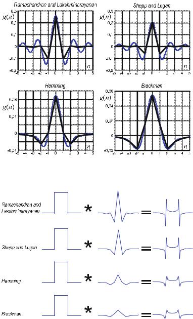
The discretized kernel of Shepp and Logan can be calculated analogously by

n sin

πn

g(n ξ) = −

− n

)

(

)

( . )

For integers, n, this yields

(

−

g(n ξ) = −(π ξ)

( . )

−

Figure . shows the discretized kernels for Ramachandran and Lakshminarayanan, Shepp and Logan, Hamming, as well as the Blackman ﬁlters. For all the ﬁlters, only

	7 Technical Implementation

Fig. . . Discretized band-limited kernels. The corresponding interpolated values of the kernels are shown as ﬁne dotted lines in the background

Fig. . . Impact of the di erent convolution kernels upon a rectangular signal. The kernels become smoother from top to bottom

7.3 Practical Implementation of the Filtered Backprojection

the value for n = is positive. Further kernels are explicitly described in Huesman et al. ( ).

For the other integer values of n, the kernel data are negative or zero. Due to the negative kernel values, blurring of the gray values of an object into neighboring regions is compensated for. Figure . shows the result of the discretized kernels applied to a rectangular proﬁle. In this ﬁgure, the kernels and the convolution results are uniformly normalized and thus directly comparable. Obviously, the ﬁlters become smoother from top to bottom.

7.3

Practical Implementation of the Filtered Backprojection

The concept of the discrete ﬁltered backprojection will once again be formulated in this section. For this purpose, let the projection signal sampled at a projection angle γn be

pγn (j ξ) with j = −D , . . ., , . . ., D − and n = , . . ., Np , ( . )

where D is the number of detector elements, which are densely packed with a distance of ξ from each other. Np is the number of projections or views.

7.3.1

Filtering of the Projection Signal

One considers the projections, pγn (j ξ), measured under the projection angles, γn , and applies a high-pass ﬁlter at each γn . This corresponds to a multiplication of Pγ (k q) with k q in the frequency domain. The periodicity of the signal Pγn (kn q) must be taken into account here (cf. Fig. . ). In MatlabTM the D frequency values are, for example, distributed such that the ﬁrst value corresponds to

Fig. . . Due to the sampling process, the spectrum of the projection signal is a periodic one. This must be taken into account when the signal is actually ﬁltered in the frequency domain

7 Technical Implementation

Fig. . . Processing chain of the raw data. As a ﬁrst step, the measured intensity is converted by logarithmation into the Radon space, the sinogram. Along the detector variable, ξ, one performs the one-dimensional Fourier transform for each projection angle, γ, and then weights each projection by multiplying it with the linear ramp q in the frequency domain. The onedimensional inverse Fourier transform along the q coordinate then yields the required ﬁltered projection

the zero frequency quantity (i.e., the DC part at frequency q = ). T hen, the positive values range up to k = D − . One ﬁnds the negative share of the spectral values seamless, i.e., the value k = D corresponds to the frequency q = −Q. If one wants

7.3 Practical Implementation of the Filtered Backprojection

Fig. . . a In general, the value of the ﬁltered projection signal to be backprojected must be calculated by interpolation since the vector r points toward the grid position (x, y)T , which yields a value ξ in the projection on the ξ -axis ranging between the values j ξ and (j+ ) ξ. b, c show the projection and the related ﬁltered backprojection under a single projection angle γ = . T he complete Radon space data are illustrated in the previous Fig. .

to implement the multiplication of Pγn (k q) with k q in the frequency domain, the di erent intervals must be properly distinguished using MatlabTM . Figure . illustrates, once again, the whole signal processing chain from the measured inten-

	7 Technical Implementation
	sity to the ﬁltered projection, based on real CT data of an abdominal section (cf.
	Fig. . ).

7.3.2

Implementation of the Backprojection

For an angle γn , every pixel in the

(

x, y

)

plane corresponds to the projection onto

the detector axis ξ via the relation

γn(

ξ ),

(

)

nξ

x cos

γn

y sin

γn

( . )

The high-pass ﬁltered projection signal, h

has to be plotted versus the projec-

tion axis, ξ, for every angle, γ

which is again given in the Hessian nor-

n . Along line LT,( )

nξ

ξ , the correspond-

mal form ( . ) by all data points r

x, y

satisfying

ing values h

γn

ξ are now to be

plotted into the spatial domain of the data points

(

)

= (

)

γn

(

) =

(

) +

(

)

x, y

j ξ is=

x cos

y sin

for all

( )

γn)

does not necessarily result in a value ξ, where h

directly available. Fig-

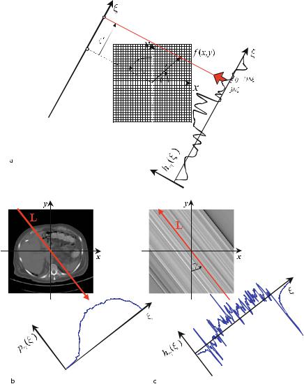
ure . a illustrates this situation. The

corresponding h

can then be derived,

(

for instance, by means of interpolation (e.g., nearest

neighbor, linear, cubic, spline,

(

)

etc.).

Thus, the ﬁltered projection is “smeared” in a reverse direction over the spatial domain under the projection angle γn , i.e., along the original X-ray beams.

Figure . b shows the original projection for a tomogram of the abdomen with the projection angle γ = . Figure . c provides a single corresponding “smearing” in reverse direction of the ﬁltered projection signal. This has to be done for all angles, γn , and these backprojections must consecutively be added.

7.4

Minimum Number of Detector Elements

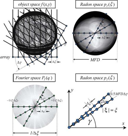
The geometrical situation, which is found during the sampling process, is illustrated in Fig. . . Without loss of generality, here the pencil-beam geometry of the ﬁrstgeneration CT scanners is used, because this geometry is easier to survey. The object space is illuminated along parallel X-ray lines with a constant angular spacing, γ. The spacing of the D sampling elements of the detector array is denoted by ξ.


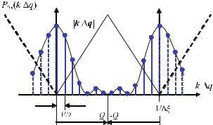
In Sect. . it has already been explained that the maximum available fre-
quency qmax in the data spectrum must be less than half the sampling rate								(	ξ	)	− ,
i.e.,
qmax <						.			( . )
				ξ
T his is theNyquist criterion. Thus, the spatial sampling interval obeys
ξ =			<
							.		( . )
	D	q			qmax

7.5 Minimum Number of Projections

The corresponding polar Radon space represents the line integrals of the scan with the geometrical location of the sampling points in the spatial domain. The diameter of the Radon space therefore directly corresponds to the measurement ﬁeld diameter (MFD) of the spatial domain. If ξ is determined by qmax, then a desired MFD yields a minimum number of detectors

	D q		D
qmax <		=		=		b Dmin MFD qmax .	( . )
			MFD		ξ

If it is assumed that the object to be reconstructed is a body with a rectangular projection proﬁle, then the spectrum is again determined by a sinc function (the ﬁrst root of which is to represent the maximum available relevant frequency).

If the object has the minimum diameter dmin, then the estimation of the max-

imum available frequency yields qmax						dmin − . This rule of thumb will be dis-
cussed again in Sect. . .			Consequently, the sampling distance is ξ D					q −
				= (		)	= (	) <
. d	min. This	results in the estimation
			Dmin		MFD
								( . )
						dmin

for the minimum number of detectors in one projection.

7.5

Minimum Number of Projections

The Fourier slice theorem ensures that the Fourier transforms of the projections are able to ﬁll up the entire frequency domain of the object. However, Fig. . shows that the distance of neighboring radial data lines in the Radon domain, (ξ, γ), just amounts to ξ γ. Therefore, the maximum distance of band-limited projections is. MFD γ. For an object with a maximum diameter dmax, the maximum distance in the frequency domain is of course limited.

With ( . ) it has been argued that

Dmin	qmax .	( . )
MFD

The number of projections is generally determined by

Np =	π
Np =	γ .	( . )

If, in addition, one takes into account the distance between the data points in the frequency domain of the individual projections, which is determined by the total length of the detector array

q =			=		,	( . )
	Dmin	ξ		MFD

7 Technical Implementation

Fig. . . Geometrical location of the sampling points in the object space, Radon space, and frequency domain. The number of required sampling points (and thus the number of detector elements D and the number of projection directions Np) is estimated by Shannon’s sampling theorem

and if it is further assumed that the maximum distance,
. MFD γ ξ ,	( . )

perpendicular to the ξ data line in the (ξ, γ) space should approximately correspond to the distance between the data points in the Radon domain of a single projection (cf. Fig. . , lower right side), then the estimation

Np =	π	π	MFD	( . )
	γ		ξ

7.6 Geometry of the Fan-Beam System

holds for the minimum number of projections. According to ( . ) the right-hand side of the estimation ( . ) thus reads

π	MFD	= π		ξDmin				,	( . )
	ξ				ξ
so that ﬁnally one obtains
Np =		π	π			Dmin
							.		( . )
		γ

As a practicable rule of thumb one ﬁnds that the requirements stipulated in the sampling theorem are met if

Np Dmin .

( . )

Due to the typically rectangular sensitivity proﬁle of detector elements, a detector quarter shift resulting in a duplication of the spatial resolution in a rotation of the sampling unit – which will be discussed in detail in Sect. . – must still be taken into account.

7.6

Geometry of the Fan-Beam System

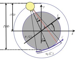
This chapter, ﬁrst of all, describes the geometry of a CT scanner of the third generation. Due to the latest developments in the ﬁeld of the two-dimensional ﬂat panel detectors, it must be assumed that the geometry of the third generation – that means a sampling unit consisting of an X-ray source and a detector array mounted on the same rotation disk – will make its way. For single-slice detector arrays located on a circular arc with the center in the X-ray focus inside the X-ray tube, the geometrical variables outlined in Fig. . play an important role.

Strictly speaking, the CT scanners of the third generation must still be subdivided into those with curved detector arrays (with equidistant angles between the detector elements) and plane detector arrays (with equidistant detector spacing). The corresponding derivations for image reconstruction with both detector types are described in the following sections.

In these systems the X-ray source moves along a circle trajectory determined by the coordinates (−FCD sin(θ), FCD cos(θ)) – as long as the CT sampling unit rotates counterclockwise, i.e., in a mathematically positive sense. Here FCD denotes the focus center distance. The angle θ is the projection angle deﬁned by the central beam. In the curved detector arrays all detector elements have the same focus center distance (FDD) from the source.

	7 Technical Implementation

Fig. . . Fan-beam geometry in CT scanners of the third generation. Curved detector arrays with constant φ are very important in clinical practice

7.7

Image Reconstruction for Fan-Beam Geometry

The conceptional philosophies of the di erent CT generations have already been pointed out in Chap. . The di erences in the reconstruction methods between the ﬁrst and the third generation will be discussed in detail in this section. Chap. described the reconstruction methods for the geometry of a pencil-beam system, i.e., for parallel X-ray beams within one projection angle. Within this geometry, the reconstruction methods are easier to understand than those for fan-beam geometry.

A serious practical disadvantage of pencil-beam geometry is, in fact, the rather di cult mechanical data acquisition process with separate rotary and shift steps, which would result in an unacceptably high data acquisition time in clinical practice. In CT scanners of the third generation, there is just one single synchronous rotation of the X-ray tube and the detector array, both of which are combined on a sampling unit, i.e., a rotating inner disk. With this construction the acquisition time is considerably reduced since the modern slip-ring technology enables a continuous rotation of the inner CT sampling unit without the previously required pauses for linear o set.

This chapter will now discuss the mathematical di erences in the reconstruction methods with respect to the transition from pencil-beam to fan-beam geometry. Figures . and . provide the di erence between the Radon spaces of a parallelbeam and a fan-beam system.

In order to ensure easily traceable projection results, the following approach is applied to a phantom consisting of two squares of di erent sizes and one circle. All objects have the same attenuation properties, thus simulating identical material.

7.7 Image Reconstruction for Fan-Beam Geometry

Fig. . . Comparison of parallel-beam and fan-beam geometry for the simple phantom consisting of three objects. The corresponding longest X-ray beam paths through the diagonal of the square objects are symbolized by thicker red lines. While these paths are found under a single projection angle with parallel-beam geometry, in fan-beam geometry these rays are obviously located in fans of di erent projection angles

On the upper right-hand side of Fig. . , a polar representation of the Radon space with parallel-beam geometry is shown. A direct comparison of the two projection geometries will be based on the Cartesian Radon spaces, which have already been introduced. The Cartesian representation of the projection values that is equivalent to the polar representation is shown on the lower left side of Fig. . . Here, parallelbeam geometry is given in a range from up to .

The data in the Cartesian Radon space are rather simple to interpret. The projections start at ( o’clock position of the tube) and, subsequently, the X-ray tube is moved in the counterclockwise sense, i.e., in a mathematically positive direction, around the phantom. First of all, at the projection of the circle is added to the projection of the large square. The projection values of the small square are separated in the projection at from the values of the other objects. Because the rotation is positive in a mathematical sense, the Radon value with the highest score is reached at (and then later in the opposite direction, which means at ).

The detector array central value, p ( ) = p ( ), is the peak value, because the longest path through the diagonals of the two square objects, arranged one behind another, has been traveled on the corresponding line of the X-ray beam. At ﬁrst glance, the Radon representations of the data are the same for both parallel-beam and fan-beam geometry. In particular, it becomes evident that for both representations the value for p ( ) = p ( ) is a peak value. The central projection is actually identical in both Radon spaces. However, di erences arise with increasing distance from the central projection.

The dashed lines in Fig. . connecting prominent points are intended to direct the eyes. These points can be easily interpreted with parallel-beam geometry at an angle of . In Sect. . the projection data proﬁles for a square object have al-

	7 Technical Implementation

Fig. . . Comparison between the Radon spaces of parallel-beam and fan-beam geometry. The upper left-hand side shows a simple phantom. It consists of two squares of di erent sizes and a circle. All objects have identical attenuation coe cients, which are homogeneously distributed. On the upper right and lower left the Radon space of parallel-beam geometry with its polar or Cartesian representation can be seen respectively. On the lower right the projection values in the Radon space of the phantom with fan-beam geometry are shown. The two lower pictures are identical only at ﬁrst glance, particularly because the highest attenuation values at and are located at the same point. With an increasing distance from the central projection, however, there are indeed di erences. A dashed line connecting prominent positions of the diagonal lines passing through the objects in the two Radon space representations is intended to direct the eyes

ready been discussed. With an angle of one ﬁnds a uniform intensity throughout the rectangle proﬁle and at a corresponding triangle proﬁle.

In the Radon space of parallel-beam geometry, one ﬁnds the triangle proﬁle of both square objects at an angle of . With fan-beam geometry, this point appears earlier for the larger square and later for the smaller square. Figure . illustrates this

7.7 Image Reconstruction for Fan-Beam Geometry

phenomenon. The beams with the longest paths through the diagonal lines of the square objects are located inside one projection angle with parallel-beam geometry. However, within fan-beam geometry one never ﬁnds the beams with the longest paths inside one fan, but in di erent fans with slightly shifted projection angles.

7.7.1

Rebinning of the Fan Beams

Figure . schematically outlines the transition from fan-beam to pencil-beam geometry. The rotation of the central beam of the fan is considered about the angle θ = θ −θ . During the rotation of the sampling unit the X-ray focus and the detector form concentric circles, which generally have di erent radii. It is obviously possible to ﬁnd an X-ray beam in the projection, ϕθ (ζ), that is parallel to one within the fan of beams, ϕθ (ζ). Synthetic pencil-beam geometry may thus be reconstructed by rebinning the corresponding beams of the fans with di erent projection angles and by recombining them.

When rebinning the fan beams, the geometrical boundary conditions must of course be carefully considered. Parameters are the fan, the aperture angle, or the length of the detector array. Figure . shows that the boundary beams of pencilbeam geometry may not be generated by rebinning with a limited aperture angle of the fan because they simply do not exist with other projection angles.

Figure . illustrates that the maximum achievable distance between the boundary beams of synthesized pencil-beam geometry, this means the distance between the ﬁrst beam ϕθ (ζ ) of the projection with the angle θ and the last beam ϕθ (ζD) of the projection with the angle θ , is directly determined by the aperture angle of the fan. This is obviously due to the fact that the related maximum change of the projection angle, θ = ψmax + ψmin, exactly corresponds to the aperture angle, φ. In

Fig. . . Left: CT scanner with fan-beam geometry. X-ray focus and detector array rotate synchronously around a common center – the iso-center in the measurement ﬁeld. Center: After one rotation of the sampling unit about the angle θ the beams in the new fan, which are parallel to the beams of the old fan, are to be found. Right: Pencil-beam geometry may be synthesized by rebinning the projection values from di erent projection angles

7 Technical Implementation

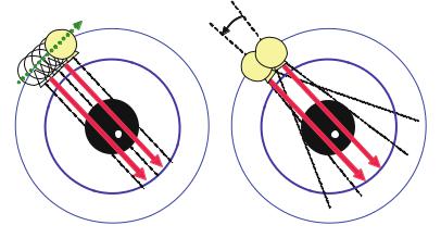
Fig. . . On the left of the picture it is shown that the maximum change of the projection angle, θ, is not independent of the aperture angle of the fan for the rebinning process. On the right the two outer parallel beams (dashed lines) cannot be generated by rebinning with a limited aperture angle

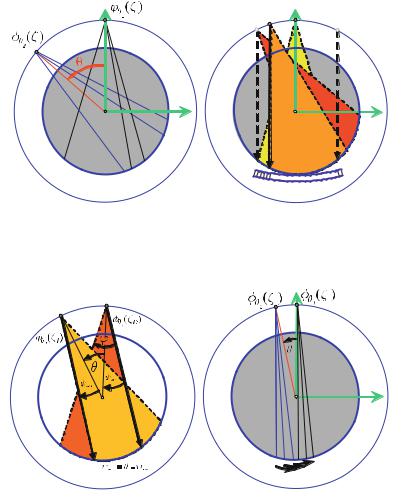
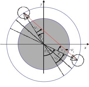
Fig. . . The maximum achievable distance between the outer boundary beams of the synthesized pencil-beam geometry is limited by the aperture angle, φ, of the fan. The related maximum change of the projection angle, θ = ψmax + ψmin, just corresponds to the aperture angle. On the right of the picture it can be seen that the pairwise parallel beams from two fan projections are available with the existing geometry only in the central area of the projection. However, in this case they always have the same angular displacement

Sect. . it will be demonstrated that the angle ψmin is not necessarily equal to the angle ψmax because asymmetrical detector arrangements are preferred in practice.

The pairwise parallel beams from two di erent projection angles of the fans are only found in the central area of the projection with the same angular displacement. It should be mentioned that of course two beams of a single fan projection may never be related to the same projection angle of the synthesized pencil-beam

7.7 Image Reconstruction for Fan-Beam Geometry

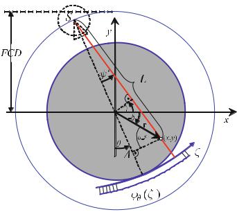
Fig. . . The geometrical conditions at the transition from pencil-beam to fan-beam geometry and vice versa. Any value of the projection, ϕθ (ζ), on the curved detector, which is characterized by the arc angle, ψ, and thus ﬁnally by the arc length, ζ = FDD ψ, must be related to a virtual linear detector. This is how a parallel projection, pγ (ξ), can be synthesized

projection. In order to be able to calculate which beam ζ in the fan projection ϕθ					ζ
corresponds to which beam ξ in the parallel projection p		γ	ξ , both systems	have
					( )
to be compared with the same ﬁgure (cf. Fig. . ). In	order to be able to measure
			( )

both projections as a function of a line section (detector arc length, ζ, or linear detector length, ξ) one will have to di erentiate here between the angle, ψ, and the

corresponding position on the detector array, ζ			FDD ψ.
	In practice only the fan-beam projection ϕθ= ζ is measured and thus known.
The projection angle for the parallel		projection is – as already mentioned in
			( )

Sect. . – the angle, γ, between the virtual linear detector axis, ξ, and the x-axis.

Due to the curvature of the detector array, the projection angle in fan-beam geometry is the angle, θ, between the central beam of the fan and the y-axis.

Considering Fig. . , one will now have to ﬁnd the relationship between the piercing point, ξ, of the virtual linear detector array under the projection angle, γ, with the projection point, ψ (ψ is an angle coordinate), of the real curved detector

array under the projection angle, θ. T his obviously obeys
and, in analogy,	ξ = FCD sin(ψ)	( . )
	FDD ψ.	( . )
Taking into account the curvature ofζthe= detector, one ﬁnds the angular relationship
	γ = θ + ψ	( . )

7 Technical Implementation

or, equivalently,

ψ = arcsin

( . )

and

FCD

This directly yields

θ = γ − ψ .

( . )

or, inversely,

ϕθ (ζ) = ϕθ (FDD ψ) = pθ+ψ (FCD sin(ψ))

( . )

pγ (ξ) = ϕγ−ψ(ζ)

( . )

= ϕγ−arcsin

FDD arcsin FCD

FCD

Fig. . . Location of the data in the Radon spaces of the corresponding geometries for small aperture angles of the fan such that the sine or the arcsine are not yet perceptible. The circles reﬂect the sampling points of the projection values on the curved detector array, ϕθ (ζ), (upper graphic) or an imaginary parallel projection, pγ (ξ), (lower graphic) respectively. According to ( . ) through ( . ), it is evident that the angle interval in which projections are acquired in fan-beam geometry must be larger than π by the aperture angle, φ, of the fan. This ensures that a complete set of values can be interpolated in the Radon space of the parallel projection

7.7 Image Reconstruction for Fan-Beam Geometry

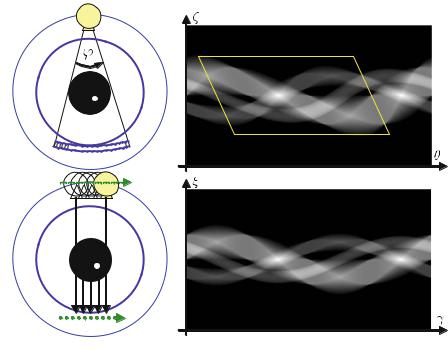
Figures . and . show the location of the data in the Radon space schematically. It is thus possible to calculate a parallel-beam projection based on the fan-beam projection by rebinning. However, it immediately becomes obvious that the measured fan projection must be interpolated. In particular, two facts have to be taken into account in this context. First of all, the calculated data points of the parallel projection are not equidistant and, unfortunately, the measuring interval required for a real parallel projection


γ , π			( . )
does not su ce to interpolate a complete; [ Radon]		space derived from the fan-beam
projection. In fact, data must be measured within the angle interval
θ ψmin , π	ψmax .		( . )
Compared with parallel-beam geometry,; [	the+ required]		measuring interval of fan-

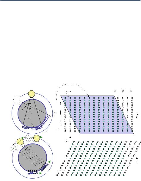
beam geometry is increased by the aperture angle of the fan, i.e., by φ = ψmax +ψmin. In Fig. . the data required for the reconstruction are highlighted in blue.

Certain boundary conditions must be taken into account to ensure fast rebinning of the sample values. Let θ and γ be the angular intervals in which a fanbeam or a parallel-beam proﬁle is measured respectively. Let these intervals obey

θ = γ = φ . ( . )

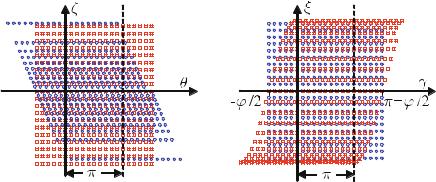
Fig. . . Locations of the data points in the Radon spaces with respect to the di erent geometries even for a very large (in practice not feasible) aperture angle of the fan. On the left, the regular grid of the (ζ, θ) Radon space is indicated by squares. Diagonal to it, the data points necessary for the calculation of the Radon space of the synthetic parallel-beam system overlaid by circles can be seen. On the right the regular grid of the (ξ, γ) Radon space to be calculated (indicated by circles) can be seen. Diagonal to it, the actual data measured by the fan-beam system, which has been overlaid with squares, are shown. The characteristic sine function stands out

7 Technical Implementation

Fig. . . The Radon spaces for fan-beam geometry (top) and parallel-beam geometry (bottom) are illustrated by a simple phantom over

Then, one may write for integer numbers n, m
ϕm φ (FDD n φ) = p(m+n) φ (FCD sin(n φ)) .	( . )

According to ( . ) the nth beam in the mth fan projection is equal to the nth beam in the (m + n)th parallel projection. The resultant, generated parallel beams are of course not equidistant and, therefore, an interpolation on the ξ-axis is necessary. Figure . once again shows the relationship between parallel-beam and fan-beam geometry of the data in the Radon space of the software phantom introduced in Fig. . .

7.7.2

Complementary Rebinning

From a physical point of view, there is no di erence in the overall attenuation of the X-ray beam caused by the tissue on its way forth and back, so the following equality applies:

pγ (ξ) = pγ π (−ξ) .

( . )

7.7 Image Reconstruction for Fan-Beam Geometry

Within parallel-beam geometry the object is therefore entirely sampled after half a rotation. For fan-beam geometry, however, an analog relationship can be established, since two beams are identical if their angles obey

In this case one ﬁnds	θ = θ + ψ $ π .	( . )
	ψ = −ψ .	( . )

Figure . illustrates these angular conditions.

If the above fact is taken into account in ( . ) through ( . ), then Fig. . can be used to ﬁnd

ϕθ	(	ζ	) = pθ+ψ (π			FCD(	ψ	))			( . )
			=	ϕθ+ ψ π(−		ζ .		(	ψ	))
			=		(− )		sin		ψ
			=		(− )

This is how a complementary X-ray source can be constructed. Figure . schematically shows the formation of the complementary X-ray source.

One may now use this knowledge concerning sampling geometry to further ﬁll up the Radon space. Based on the interval ( . ), the complementary projection

Fig. . . In fan-beam geometry there are beams within the fans of the second half of the full rotation where the paths back and forth are identical with respect to their overall attenuation

	7 Technical Implementation

Fig. . . Construction of a complementary X-ray source resulting from the physical symmetry of the attenuation path of the radiation

angle interval is obviously

π − ψmax θ π − ψmin .

( . )

7.7.3

Filtered Backprojection for Curved Detector Arrays

A practical disadvantage of the rebinning process discussed in the previous section is the fact that the reconstruction may not take place until a su cient number of fan-beam projections have been measured to synthesize a parallel-beam projection. The reconstruction process can not, therefore, run synchronously to the sampling process, but rather must wait for a certain set of measured data. Hence, it represents a bottleneck in the reconstruction chain. Furthermore, rebinning of the Radon space generally requires a non-negligible, time-consuming interpolation; therefore, one might alternatively also consider how a direct ﬁltered backprojection for fanbeam geometry might look. For this purpose one usually starts from the ﬁltered backprojection of pencil-beam geometry (Horn ; Kak and Slaney ; Schlegel and Bille ), i.e.,

7.7 Image Reconstruction for Fan-Beam Geometry

f (x, y) =

π	+		(		)
∫ −			(		)
	∫	Pγ		q		e πiq ξ	q	dq dγ
π	+		(q)e πiq(x cos(γ)+y sin(γ)) q dq dγ
∫	∫	Pγ	(q)e πiq(x cos(γ)+y sin(γ)) q dq dγ						( . )

−

π+

∫∫ Pγ (q)e πiq(rTċnξ ) q dq dγ .

−

Here, one replaces the frequency representation of the projection Pγ (q) by the explicit Fourier transform of the spatial projection signal pγ (ξ), i.e.,

(

x, y

) =

(

)

e− πiq ξ

dq dγ .

( . )

− −

∫ ∫

∫ pγ

dξ ! e πiq ξ

Changing the integration order one ﬁnds

+ +

(

)

(

x, y

) = ∫

∫ ∫ pγ

e− πiq ξ e πiq rT ċnξ

dξ dq dγ

− −

( . )

+ +

(

)

∫ − −

∫ ∫ pγ

e πiq rT

ċnξ −ξ

dξ dq dγ .

At this point, one concentrates on the integration over the frequency variable q, i.e.,

(

) =

π +

(

)

−

x, y

∫ ∫ pγ

∫

e πiq rTċnξ −ξ

dq! dξ dγ .

( . )

The bracket term in integral ( . ),

−

nξ

∫

e πiq rTċnξ −ξ

dq ,

( . )

is the ﬁlter, or convolution kernel in the spatial domain, which must be considered as a distribution (Schlegel and Bille ). This is based upon the fact that the integral ( . ) cannot be directly evaluated due to di culties related to the convergence that have been already mentioned in Sect. . . However, as a distribution within another integral, ( . ) may lead to meaningful results. Substituting the left side of ( . ) into ( . ) leads to the following convolution:

7 Technical Implementation

(

) =

(

)

−

( . )

∫

−

x, y

∫ pγ

nξ

dξ dγ

∫

(

)

−

∫ pγ

nξ

dξ

! dγ ,

which is deﬁned in the second line of ( . ) for a backprojection over .

At this point, the transformation of the coordinates to fan-beam geometry is to be carried out, which means that one has to change the coordinates:

(ξ , γ) (ζ, θ) . ( . )

When the integration variables are substituted, one is ﬁrst and above all interested in the change in the inﬁnitesimal area element, dξ dγ, during the coordinate transformation. As already discussed in Sect. . and Fig. . , the new area element must be multiplied by the Jacobian. This means that the area element, dξ dγ, is determined in the new coordinates by J dζ dθ where J is given by

∂ξ

∂γ

det

∂ ξ , γ

∂ζ

( . )

(

)

∂θ

∂(

ζ, θ )

∂ξ

∂γ

Direct substitution of the transformation equations ( . ) through ( . ) yields

∂

FCD sin

∂

FDD

∂ζ

∂θ

∂

FCD sin

FDD

∂

(

)

( . )

FCD

cos

FDD

HFCD

FCDH

cos

cos (ψ) .

FDD

Thus, the inﬁnitesimal area element is replaced during the coordinate transformation ( . ) with

dξ dγ	FCD	cos	ζ	dζ dθ .	( . )
	FDD		FDD

7.7 Image Reconstruction for Fan-Beam Geometry

If the arc angle, ψ, is used instead of the arc length, ζ, one analogously ﬁnds

dξ dγ FCD cos (ψ) dψ dθ .

( . )

To understand how the inner product (rTnξ) appears in the new coordinates, one may deﬁne the points on the backprojection lines in polar coordinates. Figure . illustrates the geometrical situation. The point r = (x, y)T is given by the equations

	x	=		r cos δ
With		=			( )	( . )
	y	= r sin			(δ ) .	( . )
	nξ	=		cos γ		( . )
		=			#
			sin(γ) ! ,
the inner product determined by the addition( )law for the cosine,
	cos(α $ β) = cos(α)cos(β) % sin(α)sin(β) ,					( . )

Fig. . . New variables are introduced for the ﬁltering process into the coordinate system of the fan beam. L is the distance between the point r = (x, y)T and the X-ray source. The point r = (x, y)T is characterized by its distance to the center of rotation, r, and the angle δ

7 Technical Implementation

reads

rT ċ nξ

					cos γ					( . )
= (r cos(δ), r sin(δ)) sin(γ)!										( . )
= r cos(γ)			δ	(. ) +	(		(	)	)
r cos	δ		cos	γ	r sin	δ		sin#γ
=	(	− )

With the new coordinates ( . ) thus reads f (r, δ)

ψmax

(

)

(

−

) −

(

))

(

)

ψmin

∫

ϕθ

FDD ψ

r cos

FCD sin

FCD cos

dψ! dθ

#( . )

and, taking into account the angle relationship ( . ), this yields

f (r, δ)π

ψmax

(

)

(

−

) −

(

))

(

)

ψmin

∫

ϕθ

FDD ψ

r cos

FCD sin

FCD cos

dψ! dθ .

( . )

This, the argument of the kernel,

g = g (r cos(θ + ψ − δ) − FCD sin(ψ)) ,

( . )

shall be examined more closely. Using the addition law ( . ), one may write

)

r cos

(

−

) −

FCD sin

(

) =

r cos

(

−

)

cos

(

) −

r sin

(

−

)

sin

(

FCD sin ψ

(

)

( . )

(

−

)

r−cos

δ(

cos ψ

(

)

) +

)

(

)

− (

sin

−

FCD

sin

As indicated in Fig. . , L denotes the distance between the X-ray source and the point r = (x, y)T. If one considers the rectangular triangle formed by the points S, A, and r, then simple trigonometry yields

and	L cos(ψ ) = FCD +r sin(θ − δ)	( . )
	L sin(ψ ) = r cos(θ − δ) .	( . )

7.7

Image Reconstruction for Fan-Beam Geometry

In Fig. . , it can be seen that

L = c

(FCD +r sin(θ − δ)) + (r cos(θ − δ))

( . )

L = c

(FCD −x sin(θ) + y cos(θ)) + (x cos(θ) + y sin(θ))

( . )

Here, ψ is a certain angle of the fan arc angle coordinate, ψ, determined by the point

(r, δ) and the projection angle, θ. This special angle is determined by

(

−

)

arctan

r cos θ

( . )

FCD

sin θ

)

−

)(

FCD −x (

)(+) +

(

)

arctan

x cos

y sin

( . )

sin

y cos

Thus, substituting ( . ) and ( . ) into ( . ) or ( . ) respectively, one ﬁnds

g = g (L sin(ψ )cos(ψ) − L cos(ψ )sin(ψ)) .

( . )

With the addition law,

sin(a − b) = sin(a)cos(b) − cos(a)sin(b) ,

( . )

the argument of the kernel, g, reduces to

g = g (L sin(ψ − ψ)) .

( . )

If one substitutes this expression into ( . ), one ﬁnds

(

) =

ψmax

(

))

(

−

))

(

)

ψmin

r, δ

∫

pθ+ψ

FCD sin

L sin

FCD cos

dψ! dθ

#( . )

(

) =

ψmax

(

)

(

−

))

(

)

ψmin

r, δ

∫

ϕθ

FDD ψ

L sin

FCD cos

dψ! dθ .

( . )

7 Technical Implementation

The inner integral again represents a convolution. Since the function g in ( . ) is the spatial convolution kernel of the linear frequency ramp, thus

	(		) =	+
	(		) =	−
g		ξ		∫	q	e πiq ξ dq ,	( . )

one may substitute here the arguments found for fan-beam geometry, so that

(

)) =

−

L sin

∫

e πiq(L sin(ψ))

The substitution

q =

sin

(

)

then yields

g (L sin(ψ)) = L sin(ψ)

−∫ q e π

dq . ( . )

( . )

iψq dq .

( . )

The integral term in ( . ) is just the desired Fourier transform of the linear frequency ramp. However, instead of the linear spatial detector variable, ξ, the angle coordinate, ψ, plays the main spatial part here. The following relationship thus applies:

g (L sin(ψ)) = L sin(ψ)

g(ψ) ,

so that ( . ) ﬁnally reads

(

) =

ψmax

(

)

(

−

)

(

)

ψmin

r, δ

∫

ϕθ

FDD ψ

g˜ ψ

FCD cos

dψ! dθ ,

where

g(ψ) =

sin(ψ)

g(ψ) .

( . )

7.7 Image Reconstruction for Fan-Beam Geometry

In analogy to the ﬁltered backprojection in Sect. . , ( . ), one may now write the short expression

f (r, δ) =	π	L hθ (ψ)dθ .
	∫		( . )

( . ) can be interpreted in such a way that the reconstruction with fan-beam geometry is a weighted ﬁltered backprojection, where

	˜	˜	(ψ)
with	hθ (ψ) = ϕθ (ψ) > g		(ψ)	( . )
	˜			( . )
	ϕθ (ψ) = ϕθ (FDD ψ)FCD cos(ψ) .			( . )

In analogy to Sect. . , Scheme . , again the reconstruction instructions should be given in an overview scheme. T he direct fan-beam reconstruction may be subdivided into three steps as shown in Scheme . .

Scheme . Filtered backprojection in fan-beam geometry for the curved detector array

. Pre-weighting of the fan-beam projection signal

˜
ϕθ (ψ) = ϕθ (FDD ψ)FCD cos(ψ) .
. Filtering of the projection signal. The ramp ﬁlter
g(ψ) =	sin(ψ)		g(ψ)
g(ψ) =	sin(ψ)		g(ψ)
˜		ψ
˜

is a modiﬁed version of the ﬁlter for the parallel projection g ψ . Combined with

	the pre-weighting process described in the ﬁrst step, the signal for backprojection
		( )
	results here from the convolution in the angular domain,
	˜	˜
	hθ (ψ) = ϕ	˜
	hθ (ψ) = ϕ	θ (ψ) g(ψ) .

. Finally, the backprojection is deﬁned over the full angle of π:

	π
f (r, δ) =	∫ L hθ (ψ)dθ .

It can be seen as a ﬁltered backprojection that is converging onto the source point in the X-ray tube. Therefore, the signal is weighted by the reciprocal squared distance between the source and the actual pixel.

	7	Technical Implementation
	7.7.4
	Filtered Backprojection for Linear Detector Arrays
	The reconstruction process based on the ﬁltered backprojection with data of a lin-
	ear instead of a curved detector array can be derived in analogy to the steps given
	in the previous chapter. Presently, in clinical practice linear arrays are of secondary
	importance. In addition, the geometrical conditions regarding the circular curved
	arrays are simpler and better adapted to reconstruction geometry because all X-ray
	paths within the fan are of the same length. However, it will be worthwhile under-
	standing the geometrical situation of the backprojection based on linear detector
	arrays, because this is similar geometry to the case of cone-beam CT (described in
		Sect. . ), which is employed with a ﬂat-panel detector matrix.
		In a curved detector array the arc angle corresponds to a circular arc length,

with the center located in the X-ray source, and the individual detector elements arranged in an equidistant angular pattern. Contrary to the above, one can just assume equidistant detectors in a linear detector array, since the corresponding angular change is non-linear. To illustrate this, Fig. . shows the geometrical situation.

Fig. . . For ﬁltering in the coordinate system of a fan beam with linear detector array, it will be necessary to introduce new variables. L is the distance between a point, r = (x, y)T, and the X-ray focus. The point r = (x, y)T is characterized by its distance, r, to the center of rotation and by the angle δ. T he variablea marks the location of a virtual linear detector in the center of the measuring ﬁeld. ϕθ (a) is the measured projection value on the virtual detector and θ denotes the projection angle of the center beam of the fan-beam projection

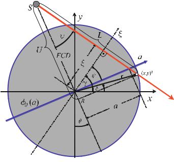
7.7 Image Reconstruction for Fan-Beam Geometry

ϕθ (a) is the measured projection value, where the variable a denotes the position on the linear detector and θ the projection angle of the center beam. Many authors do not refer to the real detector, but rather to a virtual detector placed in the origin. This concept will also be used here. Similar to the geometry of the curved array, L is the distance between a point, r = (x, y)T, and the focus inside the X-ray source. The point r = (x, y)T is characterized by its distance, r, from the center of rotation and by the angle δ.

If one assumes parallel-beam geometry for the point r, one would ﬁnd the parallel projection pγ (ξ) under the projection angle γ at detector position ξ. T heξ coordinate is shown as a dashed line in Fig. . and, by deﬁnition, it runs perpendicular to the related X-ray beam. In analogy to ( . ) and ( . ), the relationship with the fan-beam coordinates obeys

ξ = a cos(ψ) = a

FCD

( . )

and

a + FCD

γ =

θ + ψ = θ + arctan

( . )

FCD

At this point, the transform of the equation of the ﬁltered backprojection,

(

) =

(

)

(

−

)

x, y

∫

∫ pγ

nξ

dξ! dγ ,

( . )

into fan-beam geometry has to be carried out again, i.e., one has to substitute the coordinates of parallel-beam geometry with those of fan-beam geometry:

(ξ, γ) (a, θ) . ( . )

Again, the new inﬁnitesimal area element must be multiplied with the Jacobian for integration. This means that the old area element, dξ dγ, is determined in the new coordinates by J da dθ where J is given by

						∂ξ	∂γ
			(	) =		∂θ	∂θ
		∂ ξ, γ				∂a	∂a
J	det	∂	(a, θ)		H	∂ξ	∂γ	.	( . )
								H
								H

7 Technical Implementation

If one directly substitutes the transformation equations ( . ) and ( . ) one ﬁnds

∂a+

∂a

FCD

∂

FCD

∂ θ

arctan

∂

FCD

(

)

a +FCD

∂

( . )

∂θ

FCD

(

)

FCD

cos

ψ .

FCD

Thus, the inﬁnitesimal surface element is changed by the coordinate transformation ( . ) by

dξ dγ

FCD

da dθ .

( . )

FCD

If, in addition, one again takes advantage+of the relationship

one ﬁnds the expression

rT ċ nξ

= r cos(γ − δ) ,

( . )

π−arctan

amax

FCD

r, δ

pθ+ψ

FCD

. . .

(

) =

−

FCD

/−

arctan∫

. a∫min

FCD

a FCD

0 arctan

( . )

FCD −

− 6

. . . ċ g r cos θ +

FCD

daB dθ

FCD

for the ﬁltered backprojection in the new coordinates. Within this expression, the following simpliﬁcations can be implemented immediately. The limits of integration of the new angle coordinate θ had to be changed as a direct consequence of the substitution. However, since the integration over the full angle π is invariant to a constant phase shift, it is also possible to integrate in the case of this new variable from to π. Furthermore, the projection value, pγ (ξ), can be much easier expressed by means of the new detector variables since the coordinate transform yields

FCD	= ϕθ (a) .
pγ (ξ) pθ +ψ a 6a + FCD	= ϕθ (a) .	( . )

a + FCD

7.7 Image Reconstruction for Fan-Beam Geometry

( . ) is thus simpliﬁed to read

(

r, δ

) =

π - +amaxϕθ

(

)

r cos

arctan

/−

∫ . a∫min

ċ 6

. . .

FCD

daB dθ .

FCD

a	− δ −	6	a FCD			ċ . . .
FCD
			a	+	FCD
						( . )

For convenience, one substitutes the argument of the convolution kernel g with

a	,
ψ = arctan FCD	,	( . )

which can easily be understood from Fig. . . Then, addition law ( . ) can be used to calculate the argument of g with the following expression:

r cos(θ + ψ − δ) −

a FCD

FCD

) −

(

−

)

(

) − 6a + FCD( . )

(

−

)

(

r cos θ+

cos

r sin

sin

a FCD

With the expressions – which also may be read from Fig. . –

cos(ψ) =

FCD

( . )

and

a + FCD

sin(ψ) =

( . )

a + FCD

( . ) is further modiﬁed to read

r cos(θ + ψ − δ) −

a FCD

FCD

= r cos(θ − δ)

− r sin(θ − δ)

FCD

= r cos(θ − δ)

− (r sin(θ − δ) + FCD) 6

a + FCD

−6 a FCD

+( . )

a FCD

7 Technical Implementation

In analogy to ( . ) some authors (e.g., Turbell [ ]) introduce the distance

U = FCD +r sin(θ − δ)	( . )
or in analogy to ( . )
U = FCD −x sin(θ) + y cos(θ)	( . )

(cf. Fig. . ) . Similar to ( . ), one considers, with the coordinate a, the special position on the virtual detector determined by the point (r, δ) and the projection angle, θ. This very detector position is denoted a , so that

tan

) =

r cos

and thus

(

−

)

(

FCD

sin

FCD r ( − )

FCD

(

− )

)

(

− )

FCD

r cos θ

FCD r cos θ

)(+) +

sin

FCD −x

(

)(

) =

x cos

(

) +

y sin

(

)

FCD

x cos

y sin

FCD

sin

y cos

( . )

Hence, the argument of g in ( . ) can be simpliﬁed to read

r cos(θ + ψ − δ) −

a FCD

= U

− U

( . )

FCD

so that ( . ) is given by

(

r, δ

) =

π - +amaxϕθ

FCD

daB dθ .

(

)

(

−

/−

FCD

∫ . a∫min

( . )

The inner integral again represents a convolution. One should remember that the function

		(		) =	+
		(		) =	−
	g		ξ		∫	q	e πiq ξ dq			( . )
								=	FCD +r sin(θ − δ)
Occasionally, the distance is also deﬁned as the ratio UKS									FCD +r sin(θ − δ)	(Kak and
Slaney ).									FCD

7.7 Image Reconstruction for Fan-Beam Geometry

is the spatial convolution kernel of the linear frequency ramp. Here, one substitutes the new variables found for fan-beam geometry with the linear detector, thus

(	−	)6a + FCD		+
				=−		πiq(a	−a)
g	a a		U	∫	q e

The substitution

q = q 6 U

a + FCD

then yields

U	dq .
a +FCD

FCD

πiq

a a

(

−

)

−

(

− )dq

FCD

∫

and ( . ) thus ﬁnally reads

g(a − a)

(

) =

+amax

(

)

FCD

(

−

)

/−

r, δ

ϕθ

FCD

daBdθ

FCD

∫ . a∫min

/−

amax

( ) ( − ) 6

FCD

∫

ϕθ a g a

daBdθ

FCD

. a∫min

FCD

/−

amax

( ) 6

( − ) C

ϕθ

FCD

g a

a daBdθ

∫

FCD

. a∫min

( . )

=	π	U	& ϕθ (a)6a + FCD > g(a)'dθ .
	∫
		FCD		FCD

In analogy to the ﬁltered backprojection in Sect. . , one may now write the short expression

f (r, δ) =	π	FCDU hθ (a)dθ ,
	∫		( . )

7 Technical Implementation

where
hθ (a) =	ϕθ (a)	6	FCD	> g(a) .	( . )

			a + FCD

The reconstruction instructions may again be divided into three steps listed in Scheme . .

Scheme . Filtered backprojection with fan-beam geometry for the linear detector array

. Coordinate transformation for the ramp ﬁlter: The required ramp ﬁlter

(

−

)

FCD

(

−

)

UFCD

must be exactly adapted to the form of the ﬁlter for the parallel projection

by coordinate transform.

. Filtering of the projection signal: The signal for backprojection results

from the convolution

(a)6a

+ FCD > g(a)

hθ (a) = ϕθ

FCD

in the spatial domain of the linear detector.

. The backprojection over the angle π results from

f (r, δ) =

∫

FCD

hθ (a)dθ ,

which means that the projection of the high-pass ﬁltered detector signal in the reverse direction converges toward the focus of the X-ray source. While backprojecting, the signal must be weighted with the squared reciprocal variable U. In this case, U is the projection of the distance between the focus of the X-ray source and the current point onto the center beam of the fan.

7.7.5

Discretization of Backprojection for Fan-Beam Geometry

When dealing with the technical implementation of image reconstruction with fanbeam geometry, one has to answer the same question as described in Sect. . .

7.7 Image Reconstruction for Fan-Beam Geometry

regarding the discretization of the kernels. This is due to the fact that, here also, one has a sampling process with a ﬁnite number of sampling points, either in equiangular steps, φ, for the curved detector array (cf. Fig. . ) or in equidistant steps,

a, for the linear detector array.

As the single linear detector arrangements are of secondary importance, discretization will be discussed here in detail for the curved detector array only. Let the projection signal be sampled under a projection angle θn with a curved detector array having the form

ϕθn (j φ) with j = −D , . . ., , . . ., D − and n = , . . ., Np , ( . )

where D is again the (even) number of detector elements. These detector elements are densely packed and located within an equiangular distance of φ on a circle segment where the circle center is the focus of the X-ray source.

As in the previous section, the center beam is chosen as a reference beam and the projection angles in the fan therefore range from ψmin to ψmax; the index in ( . ) has been chosen such that ϕθn ( ) with j = is the center beam passing through the iso-center of rotation. Here, Np is the number of projections or views.

While the backprojection in parallel-beam geometry runs along parallel beams, the projection in the reverse direction has to take place along the fan beams, which converge at the focus of the X-ray source. If Figs. . a and . are compared, it can be seen that both concepts are so far analogous. Also, exactly as pointed out for parallel-beam geometry before, one cannot expect that in the calculation of the

Fig. . . Similar to parallel-beam geometry (cf. Fig. . ) the value of the ﬁltered projection signal to be backprojected must be obtained by interpolation since the vector r points to-

ward the integer grid position	x, y T, the projection of which on the ψ -axis (or the ζ-axis)
interval		[	j φ,	(	j		φ	]
generally yields a value in the (	)					+ )

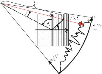
7 Technical Implementation

contribution of hθn			ψ to a certain image pixel, f		r, δ , the required value for the
angle ψ	corresponds directly to an actual, measured angle, j φ. Instead, one has to
		(		)	( )
interpolate between the sampled values.
As described in				Sect. . . for parallel-beam geometry, the kernels must also
		( . ) shows that – compared with parallel-beam geometry –
be discretized here.

one has to use a slightly modiﬁed kernel for the ﬁltering process. For convenience,

one may therefore use the discretization results found in																	Sect. . . . The discrete
sequence of the kernel ( . ) is given by
												j φ
				˜								j φ
				˜	φ) = sin(j									φ) g(j φ) .							( . )
				g(j	φ) = sin(j									φ) g(j φ) .							( . )
As g j	φ is the discretized form of the kernel for parallel-beam geometry, a com-
parison with ( . ) yields the following sequence
(	)			-
															for j =
		(					(	φ		)					for j =	(			8	)
		(	φ	) = /											for j even,	(		j	8	)	( . )
		g˜ j	φ	.	−								)		for j even,			j			( . )
				0					(				)
				.		π sin					j φ				for j odd .

Similar to the concept for parallel-beam geometry, one may use the windowing technique so that the ﬁnal result must read

˜	˜
hθn (j φ) = ϕ		( . )
	θn (j φ) > g(j φ) > w(j φ) ,

where w is the window function for which examples were given in Sect. . . . For the Shepp–Logan window this results in

gSL(j	φ) = π	φ	ctg j +	φ − ctg j − φ .	( . )
˜
˜

Due to the bracketed terms, ( . ) may also be called the cotangent kernel (Kak and Slaney ).

Similar to the previous section, one may divide the reconstruction instructions into three steps as listed in Scheme . . For the discretized version the arguments of the expressions must be replaced accordingly by the discretization ( . ) (Kak and Slaney ).

7.7 Image Reconstruction for Fan-Beam Geometry

Scheme . Discretized ﬁltered backprojection in fan-beam geometry

. Pre-weighting of each individual fan projection acquired under angle θn

˜	(j φ) = ϕθn (FDD j φ)FCD cos (j φ)	( . )
ϕθn

. Filtering of the projection signal: The modiﬁed ramp ﬁlter

			j	φ
˜
	(j φ) =	sin(j			φ) g(j φ)	( . )
g

will also be sampled in equiangular steps. The discretized convolution thus reads

˜	˜
hθn (j φ) = ϕ		( . )
	θn (j φ) > g(j φ)

. In analogy to ( . ), the backprojection over the full angle of π with angular distances of π Np is given by

f (r, δ) = ∫ L hθ (ψ)dθ

	Np				( . )
π	Np
			hθn	ψ .
Np	n =	L	hθn	ψ .
	n =			( )
				( )

This can also be seen as a ﬁltered backprojection that is converging onto the focus point in the X-ray tube. Therefore, the signal is weighted by the reciprocal squared distance between the source and the actual pixel.

An example, which can be easily understood, will illustrate the intermediate results of ﬁltered backprojection using fan-beam geometry and compare them with those of parallel-beam geometry. This example consists of a phantom with a central square of homogeneous attenuation. Figure . ﬁrst shows the Radon spaces of the object. In addition to the known Cartesian representation of the projection values, pγ (ξ), this ﬁgure also shows the Radon space with its polar coordinates on the upper right-hand side. The Cartesian Radon space of the fan-beam geometry of the square is shown on the lower right-hand side. The intensity values are the projections ϕθ (ζ).

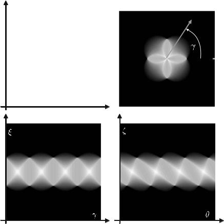
7 Technical Implementation

Fig. . . To illustrate the di erences in the Radon spaces between parallel-beam geometry and fan-beam geometry for the same object, once again a very simple phantom presented on the upper left is used here. The square object has homogeneously distributed attenuation coe cients. On the upper right and lower left, the Radon spaces of parallel-beam geometry with both their polar and Cartesian representations are depicted. Both representations are equivalent. On the lower right, the projection values in the Radon space of the phantom with fan-beam geometry are illustrated. The di erence between the two pictures on the lower side is that the data in the Radon space of fan-beam geometry are tilted

As expected, a direct comparison of the Cartesian Radon space representations results(in)a tilting of the data, ϕθ (ζ), with fan-beam geometry compared with the data, pγ ξ , of parallel-beam geometry. The data rebinning concept explained in Sect. . . can also be readily understood here. However, the projection data, ϕθ (ζ), will now be used to calculate a direct reconstruction according to ( . ) through ( . ).


		7.7 Image Reconstruction for Fan-Beam Geometry
The pictures displayed in Fig. . show the direct reconstructions with a suc-
cessively increased number, Np – cf. ( . ) second line – of the projections, ϕθ							ζ .
In this case, N		p runs through the values , , , , , . Similar to				parallel-
		p runs through the values , , , , , . Similar to					( )
		object is not displayed with a small num-
beam geometry, the true structure of the
ber of views, Np. Particularly striking is the fact that fan-beam geometry is directly
reﬂected in the backprojections. This is, thus, also a very intuitive method. The in-
dividual projections look like the light cones of a pocket lamp.
Figure . once again directly compares the ﬁltered backprojection with the
two geometries – fan-beam and parallel-beam – taking Np					as an example. In
the three-dimensional representation the speciﬁc ﬁlter			response on the rectangle
the three-dimensional representation the speciﬁc ﬁlter				=
is readily visible for both geometries. This is described by ( . ) through ( . ).
In parallel one can also recognize the quadratic decay of the single projection in
a reverse direction with increasing distance to the source. This behavior is due to
the	L normalization given in ( . ).
the	L normalization given in ( . ).

The linear detector array is discretized in the same way as the curved detector array. As g(j a) in ( . ) is exactly the discretized form of the kernel for parallel-

Fig. . . Backprojection with fan-beam geometry. Successive reconstruction of the tomographic phantom image based on the projection data. The number of projections is exemplarily increased image by image: Np = , , , , , . T he reconstruction principle is again easy to understand intuitively. The backprojected data look like the light cones of a pocket lamp

7 Technical Implementation

Fig. . . Comparison between the ﬁltered backprojection with fan-beam geometry (lefthand column) and the ﬁltered backprojection of parallel-beam geometry (right-hand column). The length-dependent scaling according to ( . ) is readily visible with fan-beam geometry. However, the characteristic ﬁlter response to the rectangle is visible in both representations

Fig. . . Similar to parallel-beam geometry (cf. Fig. . ), the value of the ﬁltered projection signal to be backprojected must be calculated by interpolation. This is necessary since the

vector r points toward the integer grid position	x, y T
generally yields a value in the interval [j a, (j	(+ ) )a], the projection of which on the a-axis

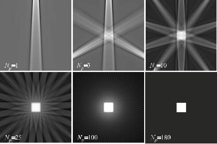
7.8 Quarter-Detector Offset and Sampling Theorem

beam geometry, one may directly apply ( . ) to ﬁnd the sequence

				-								for j =
	(			-			(	a	)			for j =	(		8	)
g	(	j	a	) = /								for j even,	(	j	8	)	( . )
g		j	a	.	−							for j even,		j			( . )
				.								for j odd
				.		π j		(		a	)	for j odd
				0				(			)

for practical implementation. Figure . shows the principle of backprojection with the required interpolation between individual detector positions.

7.8

Quarter-Detector Offset and Sampling Theorem

As described in the previous chapters, a reliable reconstruction of an object is ensured if any point of the object has been radiographed from all sides. For parallelbeam geometry, the object will of course just have to be illuminated over an angular range of . This is because – due to the physical properties of the X-ray beam – the attenuation is independent of whether the beam passes through the object in a forward (L ) or in a reverse direction (L ).

Therefore,

f > δ(L ) = ∫ f (r)δ (rT ċ nξ) − ξ dr

= pγ (ξ ) = pγ (ξ )

= R∫ f (r)δ (rT ċ (−nξ)) − ξ dr	( . )
= R∫ f (r)δ (rT ċ (−nξ)) − ξ dr
= f > δ(L )
actually just yields a mirror-inverted projection, which means
pγ (ξ) = pγ + π (−ξ) .	( . )

Figure . illustrates this issue once again. The information obtained by acquiring data over angles exceeding is thus redundant.

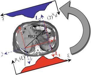
	7 Technical Implementation

Fig. . . If one illuminates an object under the angles γ and γ + π, then one ﬁnds a mirrorinverted projection with a symmetrical detector array, i.e., pγ (ξ) = pγ+π (−ξ) and thus redundant information. But if the detector array is adjusted slightly asymmetrically, it is possible that the opposite projection samples the space precisely in such a way that the total sampling rate is doubled. One may easily understand that this occurs when the detector array is set o by one-quarter of the detector width

Nevertheless, all modern CT scanners create projections covering . T his initially seems to be absurd because – from a mathematical point of view – this redundant information is not necessary, i.e., the radiation dose may be doubled unnecessarily. Therefore, the radiation dose must be lowered if the scan is carried out by choosing a reduced X-ray intensity. Noise must then be reduced in a further processing step where statistically independent noise contributions of centrally opposed projections are averaged.

Practical applications, however, use a di erent approach since the sampling theorem has consequences on the sampling process in CT. As mentioned earlier, the measurement of the attenuation values with a detector array of a third-generation scanner is, of course, a sampling process. Figure . shows the sampling situation with an array consisting of D detectors (enumerated from to D here), each having a constant detector width, ξ. The detectors are arranged in an array as densely as possible. The spatial separation of the individual elements by the anti-scatter grid will not be examined here.

Even though the integration along the X-rays represents an averaging process ﬁltering the projection signal like a low-pass, it must nevertheless be ensured that projection aliasing due to undersampling cannot occur. From a physical point of view the object is spatially continuously illuminated in the X-ray fan beam. Therefore, high-contrast edges such as transition zones at a bone/soft-tissue interface generate a large bandwidth. Hence, this yields a spatially, rapidly varying, continuous projection sampled with the detector array.

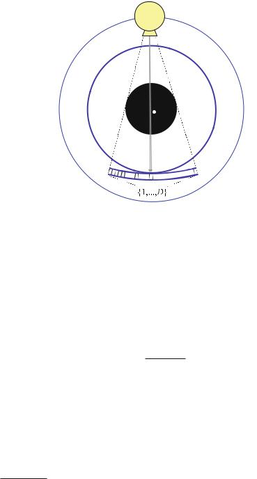
7.8 Quarter-Detector Offset and Sampling Theorem

Fig. . . A detector array with D detectors acquires the integral attenuation values. The phantom in the middle of the measuring ﬁeld has sharp-edged structures and thus produces higher spatial frequencies than the spatial frequency of the detector array. The requirements stipulated in Shannon’s sampling theorem are thus not met

As every detector element has a ﬁnite width, ξ, with constant sensitivity the measured values are averaged over this width, i.e., the measuring process already includes a natural low pass. Overall, however, the projection signal is a step function . The proﬁle of a single detector element is thus a rectangle function with a width, ξ.

As described in

Sect. . , the frequency representation of a rectangle in the spa-

tial domain is

the sinc function, i.e.,

(

)

(

)

sin

ξu

( . )

ξu

As a consequence, the measured signal is thus not band-limited so band overlap problems may arise. The essential energy contributions are included in the sinc function up to the ﬁrst root. One therefore assumes that the highest available frequency (which is relevant in practice) is determined by the ﬁrst root, given by

π ξu = π .

( . )

A similar problem will also have to be discussed in the next chapter dealing with the secondary reconstruction of a three-dimensional image from a stack.

7 Technical Implementation

This means that the maximum frequency (which is again relevant in practice) is given by

u =
u =	ξ .	( . )

However, Shannon’s sampling theorem states that the distance between the sampling points must be ξ , i.e., that they must be twice as densely arranged than is actually possible due to the structural design.

According to Shannon’s theorem, it would also be possible to ﬁlter with a low pass over two detector widths to prevent band overlap problems. However, the related deterioration of the modulation transfer function (MTF) of the system (cf.Sect. . ) would not be acceptable in clinical practice.

In fact, actual implementations do not ﬁlter over two detector elements, but increase the spatial sampling frequency with an elegant technical modiﬁcation of the detector.

The spatial sampling rate is doubled by setting the detector array o by one quarter of the detector width. This is readily illustrated in Fig. . : It can be seen that the central beams are located side-by-side at a distance of half the detector width after one rotation by .

For the o -center beams, it is assumed that the space is sampled in the measuring ﬁeld on concentric circles around the iso-center of rotation. With a symmetrical detector arrangement, one just needs a rotation around the object to image

Fig. . . Quarter detector shift in a CT scanner of the third generation. Left: Without an o - set, the way forth and back yields the same projection value due to the symmetrical attenuation and thus no new information is obtained. Right: Taking advantage of an asymmetrical detector arrangement on the way forth and back of the X-ray beam, a sampling pattern can be achieved such that the desired double sampling rate is generated

7.8 Quarter-Detector Offset and Sampling Theorem

Fig. . . Duplication of the sampling rate by a quarter detector shift to meet the requirements stipulated in Shannon’s sampling theorem. The di erences in radii of the concentric sampling circles are half as much with the quarter detector shift (right-hand images) than with the symmetrical detector arrangement (left-hand images). The principle is the same for parallel-beam geometry (the two upper pictures) as for fan-beam geometry (two lower images). Contrary to parallel-beam geometry, the distances between the sampling circles become smaller and smaller with an increasing angular distance from the central beam with fan-beam geometry

any point of the object from all sides. By setting o the detector array by one quarter of the detector width, the X-ray tube has to be rotated by around the object to illuminate any point of the object under any angle. However, this additional

7 Technical Implementation

technical e ort results in the availability of supplementary sampling circles. The lo-

cal di erence in radii of those is just half as much as for a symmetrical detector

arrangement. The spatial sampling rate has thus been doubled – as requested by

Shannon.

Figure . also illustrates that the described concept of doubling the resolution

can be put into e ect for both fan-beam and parallel-beam geometry. However, the

di erences in radii are become smaller for larger angles with fan-beam geometry,

whereas the parallel-beam system is characterized by a homogeneous resolution.

In general, this method can be used successfully if a su cient number of pro-

jections is available for a single rotation (with typical resolution limits ranging

from up to line pairs per centimeter) approximately , projections are re-

quired per rotation (Morneburg ), and if the patient movement is negligibly

small. This is due to the fact that it takes a certain time to carry out a rotation

and the complementary beams from the corresponding opposite side double the

spatial sampling process.

Figure . illustrates the rebinning of the sample points in the Radon space.

With the quarter detector shift, the sample points of the angle intervals on the back-

side π, π are just located between the sample points of the angle intervals on the

front[side [] , π]. The spatial sampling rate is thus doubled.

Fig. . . Sampling points in the Radon space (of pencil-beam geometry) with a quarter detector shift. If one correctly rebins the sample points of the angle interval [π, π] into the interval on the front side [ , π], the spatial sampling rate is doubled

7.8 Quarter-Detector Offset and Sampling Theorem

Fig. . . Sampling points in the Radon space (of pencil-beam geometry) with a quarter detector shift and with a supplementary integer detector element o set. If the sample points are properly sorted from the angle interval [π, π] into the interval on the front side [ , π], one can see that the spatial sampling rate is only doubled in the central area. This area is highlighted in gray. At the same time, one observes a synthetic extension of the detector arrays whereby aliasing problems may occur due to the single spatial resolution

7 Technical Implementation

Fig. . . As the detectors are positioned asymmetrically, measurement ﬁelds with di erent spatial resolutions are obtained. Due to the quarter detector shift, the resolution is twice as good in the inner measurement ﬁeld than in the outer measurement ﬁeld

Fig. . . Compact tomograph Philips Tomoscan M. For the outer measurement ﬁeld it immediately becomes obvious why projections must be measured over . As a result, this measuring method does indeed yield twice the resolution in the inner area

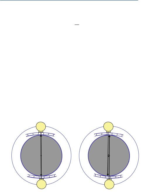
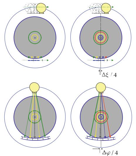
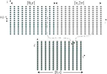
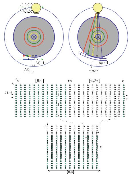
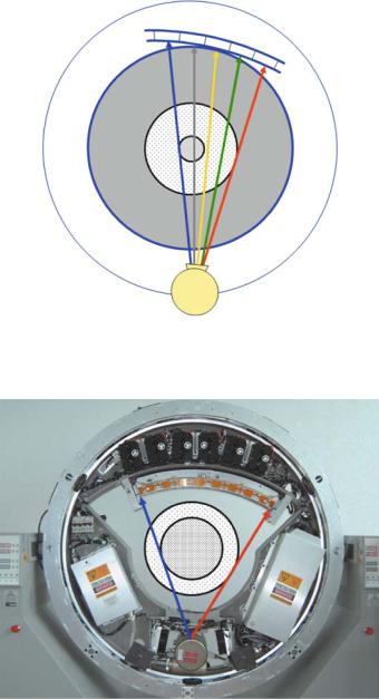
7.8 Quarter-Detector Offset and Sampling Theorem

In compact low-cost CT systems, in which the engineers try to reduce the number of detector elements, the shift of the detector array is increased even more so that ﬁnally two di erent reconstruction areas are achieved: one inner area that has twice the spatial resolution of the outer area, due to the quarter detector shift. As the outer area of the measuring ﬁeld usually covers the extremities, the corresponding loss in resolution does not play a major role in diagnostics.

Figure . illustrates the location of the sample points in the Radon space. The asymmetrical arrangement of the detector array results in a parallel o set of all points along the detector array axis. The points in the angle interval [π, π] are sorted into the angle interval [ , π] such that a central area with twice the sampling rate is generated (in Fig. . , bottom, highlighted in gray). The detector array has thus been artiﬁcially extended. However, one only obtains a low spatial resolution in the extended area so that aliasing problems may occur.

However, given that – as already mentioned above – the area that is of diagnostic interest is in general positioned in the center of the measurement ﬁeld, this e ect plays a minor role. Figures . and . show the two resolution areas schematically on a compact Philips Tomoscan MTM CT scanner. Another model of a compact scanner with asymmetrical detector array is the Siemens Somatom AR.T/CTM scanner equipped with what is called a / detector.

8Three-Dimensional Fourier-Based Reconstruction Methods

Contents
8.1	Introduction . . . . . . . . . . . . . . . . . . . . . . . . . . . . . . . . . . . . . . . . . . . . . . . . . . . . . . .	303
8.2	Secondary Reconstruction Based on D Stacks of Tomographic Slices . . . . . . . . . . . . .	304
8.3	Spiral CT . . . . . . . . . . . . . . . . . . . . . . . . . . . . . . . . . . . . . . . . . . . . . . . . . . . . . . . . . .	309
8.4	Exact D Reconstruction in Parallel-Beam Geometry . . . . . . . . . . . . . . . . . . . . . . . . .	321
8.5	Exact D Reconstruction in Cone-Beam Geometry . . . . . . . . . . . . . . . . . . . . . . . . . . .	336
8.6	Approximate D Reconstructions in Cone-Beam Geometry . . . . . . . . . . . . . . . . . . . .	366
8.7	Helical Cone-Beam Reconstruction Methods . . . . . . . . . . . . . . . . . . . . . . . . . . . . . . .	394

8.1 Introduction

In this chapter, three-dimensional reconstruction methods will be discussed. The chapter starts in Sects. . and . with a description of pseudo three-dimensional methods that are based on stacks of two-dimensional images. The spiral CT method described in Sect. . also follows this pseudo three-dimensional approach, although in this case data acquisition is actually closer to a true three-dimensional reconstruction method. In this context, the term true means that the third dimension of the images is not the result of a secondary reconstruction in which the actual, i.e., primary, reconstruction only refers to two-dimensional Radon transforms.

Methods based on three-dimensional Radon transforms will be discussed inSects. . and . . In fact, the exact reconstruction methods based on cone-beam geometry are mathematically more demanding than the two-dimensional methods discussed in Chaps. and . Although there have been studies investigating the use of algebraic reconstruction techniques (cf. Chap. ) related to cone-beam geometry, scientiﬁc interest is nowadays focused on Fourier methods, which will be exclusively addressed in this chapter.

Figure . demonstrates the tremendous development in the ﬁeld of X-ray- based imaging to date. Figure . a shows an excellent projection image in which a multitude of details of the anatomy are already visible. However, in this image

ART or the statistical reconstruction methods discussed in Chap. can be implemented in D in a straightforward manner.

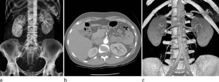
8 Three-Dimensional Fourier-Based Reconstruction Methods

Fig. . . Example of an abdominal situation illustrating the progress in imaging – starting with a a simple X-ray picture, then b the tomographic reconstruction, and in c the volumeor cone-beam CT reconstruction (courtesy of General Electric Medical Systems: Pfoh [ ])

the diagnosis is impaired due to the typical projective superimpositions. Figure . b shows a tomogram slice, which brought along a revolutionary improvement of contrast and thus of diagnostic insight. The steps to volumeor cone-beam CT are no less revolutionary. With CT scanner prototypes equipped with special ﬂat-panel detectors it is possible to show that a resolution of approximately μm can be achieved. Figure . c shows the result of such a volume scan. This high-resolution, isotropic volume representation is realized with a detector element density of approximately . elements per cm (Pfoh ).

8.2

Secondary Reconstruction Based on 2D Stacks of Tomographic Slices

In the previous chapters, only two-dimensional images have been considered. However, today, medical applications of computed tomography (CT) are mainly related to three-dimensional imaging. In a ﬁrst step, a stack of two-dimensional slices must be acquired. A conventional technique is given by a sequential procedure where the patient, laying on the patient table, is moved slightly in the axial direction of the scanner, i.e., the scanner’s z-axis. The table then stops and a complete raw data set of a single slice is measured. Figure . shows a representative result of this process. The stack of tomogram slices is subsequently used to compute the threedimensional representation of the depicted anatomy. This procedure is called secondary reconstruction.

As for the surface visualization method, it is necessary to select a gray value threshold representing the surface. In this context one has of course a certain degree of freedom, as di erent objects may be visualized as long as their Hounsﬁeld values are clearly di erent from one another. The gray-value iso-surface will then be illuminated with a virtual light source so that the corresponding light reﬂections can be computed to display the result.

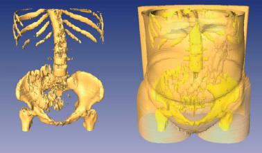
8.2 Secondary Reconstruction Based on 2D Stacks of Tomographic Slices

Fig. . . Three-dimensional visualization of the slice stack. For visualization purposes a socalled surface rendering method is used based on a gray value iso-surface representation. If one selects a su ciently high gray value threshold for the iso-surface, so that virtually only the bone structures are segmented, then the soft tissue parts obviously vanish (left). If one selects another threshold representing the soft tissue and the skin, then these objects can be visualized as well (right)

This rather simple surface segmentation method fails in all those cases in which distinct objects have very similar gray values. Therefore, it is hardly possible to identify an appropriate threshold that allows these objects to be clearly distinguished. Moreover, if the gray values vary in di erent areas of certain organs so that they cannot all be represented by a single threshold value, this method fails as well. In these unfortunately prevalent cases, one has to apply more intelligent and potentially also interactive segmentation methods. This wide range of di erent segmentation methods cannot be discussed here. A corresponding introduction is available, for example, in Lehmann et al. ( ). However, this problem will once again be addressed in Sect. . . . There it will be explained how and under which basic constraints the stack of slices is measured. Figure . shows the patient table feed as a function of the measuring time. This yields the above-mentioned stacks of slices, which, arranged side by side, result in the desired volume image.

From a signal theoretical point of view this sequential slice acquisition must again be interpreted as a sampling process. In this case, the samples are taken along the z-axis. The Nyquist criterion, which was introduced in Sect. . , must of course also be taken into account in this context.

The intensity proﬁle of the radiation in a single slice to be reconstructed, which is rectangular under ideal conditions, is restricted by a slot-like collimator in the third-generation scanners. Now let the axial width of this rectangle be z. As already discussed in Sect. . , the frequency representation of a rectangle in the

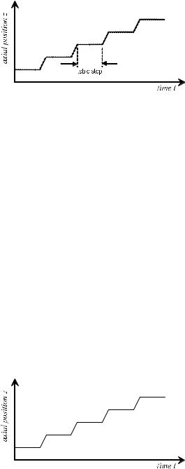
8 Three-Dimensional Fourier-Based Reconstruction Methods

Fig. . . The measurement position as a function of time. Raw data set measurements are taken each time the table stops

spatial domain is the sinc function, which means
Z w	sin π		zw		.	( . )
		π
( )	(			)

Taking into account that the essential energy contributions of the sinc function ( . ) are included in the frequency interval up to the ﬁrst root at

π zw = π ,			( . )
then the maximum frequency of the signal relevant in practice amounts to
w =
		.	( . )
	z

In order to meet the requirements stipulated in Shannon’s sampling theorem, the

distance between the sampling points must therefore be		z . This means that with
a slice thickness of z the table feed may be as much as		z . At least two slices must
therefore be measured per slice thickness. Figure .	shows the thickness of the slice
therefore be measured per slice thickness. Figure .

Fig. . . The slice thicknesses in each measuring position as a function of measuring time. The values are always measured during the stop period of the table feed

8.2 Secondary Reconstruction Based on 2D Stacks of Tomographic Slices

Fig. . . Slice stack from abdomen tomography. A sequence of successive slices is shown line by line

at any measuring position as a function of the time. Typical slice thicknesses range from mm up to mm.

This condition from signal theory is hardly taken into account in practice. In fact, many radiologists just place the slice images of a sequence side by side on their viewing light box to evaluate the radiographs quickly; thus, aliasing plays a sec-

8 Three-Dimensional Fourier-Based Reconstruction Methods

Fig. . a,b. The individual images of a slice stack are arranged one after another. This arrangement results in a volumetric representation and therefore represents the basis for CT to be considered as a three-dimensional modality. A surface rendering technique has been used here

8.3 Spiral CT

ondary part. Figure . shows such a sequence of axial slices of the abdominal region.

As already discussed above, the slices of the stack shown in Fig. . must be placed on top of each other to provide a three-dimensional representation. Figure . illustrates this procedure schematically with ﬁve single slices being arranged using the same three-dimensional data set. The tomograms are stacked one by one with exactly matching pixels . In general, the slice thickness considerably exceeds the pixel size within one slice. This means that the voxels are anisotropic, a fact that must be taken into account when algorithms of three-dimensional image processing are used, for example, by isotropizing the data set by interpolation. Nevertheless, errors might occur during visualization and data evaluation if the above-mentioned sampling theorem is violated during data acquisition. A corresponding example is illustrated in Sect. . . .

Figure . a shows ﬁve single slices together with a surface representation of the skeleton. For this purpose, the selected gray-value threshold is high enough to suppress any kind of soft tissue in the representation. In Fig. . b the skin and some organs have been segmented by applying another, smaller gray-value threshold. Correspondingly, they are visualized as transparent material.

8.3 Spiral CT

A ﬁrst step toward a true volume image is the so-called spiral CT method, which was proposed by Willi Kalender in on the annual RSNA conference (Kalender et al. ). The inadequacies of the simple slice stack produced by conventional CT are easy to understand. Due to the preset collimation each slice has a certain width, which is also referred to as slice thickness. Within this slice thickness the intensity is weighted with its sensitivity proﬁle – given by the source intensity distribution inside the collimation and the detector sensitivity proﬁle – and then averaged.

This averaging process is a problem in all those cases in which the object is characterized by boundaries, which are angulated with respect to the axial slice, i.e., where structures to be displayed quickly change in the direction of the table feed. In these cases, the averaging process results in a step-like slice stack so that the structure to be displayed has a staircase-like appearance. This artifact formation will

This only is true, if the patient holds his breath during data acquisition. Otherwise, motion artifacts appear (cf. Sect. . . ). Sophisticated image processing methods can be employed to correct for these artifacts in a post-processing step.

Voxel is an artiﬁcial word composed of volume (x) element.RSNA: Radiological Society of North America.

8 Three-Dimensional Fourier-Based Reconstruction Methods

Fig. . . Three-dimensional representation of a part of the vertebral phantom. Orthogonal reformatting, as well as volume rendering, is displayed. The slice thickness selected for the measurement is . mm. The step-like pattern of the three-dimensional rendering and of the calculated coronal and sagittal sections can be clearly distinguished

once again be discussed in Sect. . . . Figure . shows an example of this e ect by means of a volume rendering and MPR model of a vertebral phantom.

Volume rendering: Each voxel is assigned to a physical light reﬂectance and scattering. In the computer, this “data fog” is illuminated with a virtual light source and the optical events at the voxels are simulated.

MPR: Multi-planar reformatting.

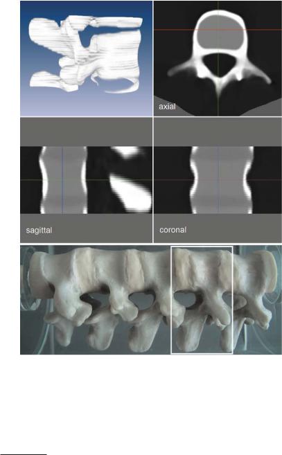
8.3 Spiral CT

The development of slip-ring technology, which has already been brieﬂy discussed in Sect. . , made it possible to rotate the sampling unit, i.e., the tube and detector array system, continuously. If the table feed is kept constant during the rotation, then the X-ray source rotates around the patient on a spiral path ; strictly speaking, this movement describes a helical trajectory. This orbit interpretation is based on a coordinate system attached to the patient table, since the X-ray source does of course still run along a circular path. The spiral path only arises from the patient’s view. With this concept, the complete projection data acquisition of an object is possible, and the scan time for a volume could be considerably reduced in comparison with conventional tomography.

Indeed, it is remarkable that spiral CT technology works at all. An essential requirement for the reconstruction methods described in Chap. is the completeness of the raw data. This means that an object in the measurement ﬁeld can only be reconstructed if all points of the object are illuminated from all sides – i.e., over (cf. Fig. . left side). This condition is the reason why artifact-free conventional CT scans of the heart are practically impossible because the heart motion shifts parts out of the slice to be reconstructed while the sampling unit rotates around the heart. Thus, the projection data to be used for the reconstruction process do not fulﬁll the consistency condition. Rather, the di erences between the projection data of a complete cycle should only be caused by the change of perspective. The reconstructed tomogram is thus impaired by motion artifacts, which will be described in detail inSect. . . .

In spiral CT scanners, the motion of the objects to be reconstructed is in fact the decisive innovation compared with conventional CT scanners. Figure . , righthand side, illustrates that the object to be examined is no longer scanned in a single plane. The reason for this is that, due to the continuous patient table feed, the source trajectory is not a closed circular orbit. Therefore, a complete set of raw data is not available for the reconstruction process – the data are inconsistent in terms ofChap. . In Fig. . , bottom, the raw data space of spiral tomography of the head is shown. During the patient table feed of cm, projection data of six full cycles of the sampling unit have been acquired. It can easily be seen how the information in the sinogram changes while the patient is moved along the z-axis.

Figure . shows the conceptual di erence between the source trajectories for the conventional and the spiral CT method for a larger volume. The conventional scanning scheme is shown on the left-hand picture. The tube moves along circular paths, which are traversed completely and pushed over the patient successively with discrete stops. Due to the ﬁnite collimation, the thickness of the slices is determined by the width of the circular path. On the right-hand side it can be seen how the circular path of the tube is combined with the continuous linear table feed in the spiral CT scanner and thus arranges the data on a helical trajectory.

A decisive di erence between the two methods is readily visible in Fig. . . In conventional tomography there are areas that are not illuminated at all with the

One should actually name the orbit a screw path because a spiral is a purely D structure in which the radius of the cycling trajectory point is linearly changed.

8 Three-Dimensional Fourier-Based Reconstruction Methods

Fig. . . Completeness of the data in conventional CT (left). Due to the continuous table feed, the raw data acquired with spiral CT are not complete. The path of the X-ray source is not a circular orbit. Below: Sinogram raw data of the head acquired with a spiral acquisition protocol

ratio of table feed and slice width illustrated above. Information required for image reconstruction is thus not available from these areas. The errors related to threedimensional visualization have already been discussed above.

This is di erent in spiral CT scanners because – as already described above – these scanners are characterized by continuous data acquisition, i.e., all points along the z-axis are illuminated at least once. Therefore, at least partial information from

8.3 Spiral CT

Fig. . . Comparison of data acquisition between conventional CT and spiral CT. Left: Due to stop points of the table feed, the data are measured on separate circles in conventional CT. Right: The combination of the continuous rotation of the sampling unit and the continuous table feed results in a helical arrangement of the raw projection data in spiral CT scanners

each slice, which can be subsequently and arbitrarily selected, will be available for the reconstruction process. And, in fact, information is even available for smaller objects from di erent projection directions over the entire width of the slice due to the speciﬁc slice sensitivity proﬁle determined by the chosen collimation.

The key idea governing the reconstruction process of the spiral CT method is based on the assumption that the missing data of one slice can be completed by interpolation. If this has been done, then the two-dimensional reconstruction procedures described in Chap. are again available without any restriction. Figure . shows the simplest principle of a slice interpolation. The helical rise, i.e., the path along which the table is moving during one rotation of the sampling unit, will be denoted with s here.

One may now select an arbitrary slice position, zr, because no preferred axial position regarding the data basis exists due to the constant table feed. For the selected slice there initially is only a single projection angle, γr, for which the pro-

Fig. . . Principle of slice interpolation in spiral CT. The corresponding neighboring projection data, which have actually been measured, contribute to the projection data of the selected slice by interpolation

8 Three-Dimensional Fourier-Based Reconstruction Methods
jection data set pγr ξ is available. The projection data pγ						ξ of all other projec-
provided accordingly by means of interpolation. For this pur-
tion angles must be( )						( )
pose, the data that have not been measured under the other required projection
angles in the selected slice position zr, must be interpolated on the basis of the
closest neighboring angles of the helical trajectory that have actually been meas-
ured.
The simplest case of such an interpolation scheme is a so-called linear interpol-
ation. For this purpose, one ﬁrst identiﬁes each position z with a projection angle,
so that
	γi =	zi
							( . )
		s					( . )
and thus
	γi + =		zi	s+ s	.		( . )
	γi + =			s+ s	.		( . )

In fact, the actual interpolation is a sum of the left-hand pγ (ξ) and right-hand pγi + (ξ) neighboring projection, each weighted with the correspondingi distance to the selected slice. That is

pγr (ξ) = ( − α)pγi (ξ) + αpγi + (ξ) ,

where the weight α is determined by	=		−
α	=	zr	−	zi	.
α			s		.
			s

( . )

The linear interpolation over an angle of already yielded remarkable success when it was introduced by Willi Kalender. This interpolation is abbreviated byLI, where LI denotes linear interpolation. Nevertheless, it should be discussed whether the interpolation might yield even better reconstruction results if the acquired data basis could be measured more densely. Figure . illustrates that the raw spiral projection data of an acquisition interval over are required for an interpolation of a single slice with the LI method.

On the other hand, it is desired to achieve a higher density of the underlying projection data without having to increase the radiation dose. To realize this, one may take advantage of the fact that the attenuation of X-ray beams along the beam path is invariant to direction reversal. This is the reason why projection data must generally only be acquired over an angle interval of in parallel-beam geometry. This means that with each measured projection proﬁle pγ (ξ), one also knows pγ+ (ξ). With this idea, a second helix is obtained, which, compared with the basic helix, has been shifted by . This supplementary helix is shown in Fig. . .

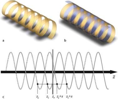
8.3 Spiral CT

Fig. . . Principle of slice interpolation in spiral CT. Due to the invariance of the attenuation to the reversal of the beam path, one obtains a supplementary helix, which is shifted by compared with the basic helix. a Simple spiral with pitch p = , b supplementary helix ﬁlling the gap, and c interpolation with data from the supplementary helix. The complementary trajectory is indicated with a dashed line

The supplementary helix is generated regardless of whether parallel-beam geometry is considered or the fan-beam geometry of the third-generation tomographs, which are used mostly nowadays. In Sect. . . , it has already been mentioned that an inverse fan can be synthesized by complementary rebinning, which also describes a supplementary helix.

The beneﬁt of the complementary helix is easy to understand. The data points for the interpolation are much closer to each other without increasing the radiation dose. Figure . c illustrates that now the points zi and zj + s are the nearest points for the approximation of the projection data point zr. The frequently applied LI method uses the supplementary helix in a linear interpolation scheme. Overall, raw projection data from an acquisition interval of ( +φ) are required to carry out the interpolation in a fan-beam system with the LI method. In Sect. . , it has already been discussed that one has to measure by the aperture angle φ of the fan beam beyond if fan-beam geometry is used instead of parallel-beam geometry to acquire a complete Radon space.

In addition, one may carry out a higher order interpolation if the points zj and zi + s indicated in Fig. . c are considered as well. However, this issue will not be discussed in detail here. A survey of the interpolation algorithms used in CT

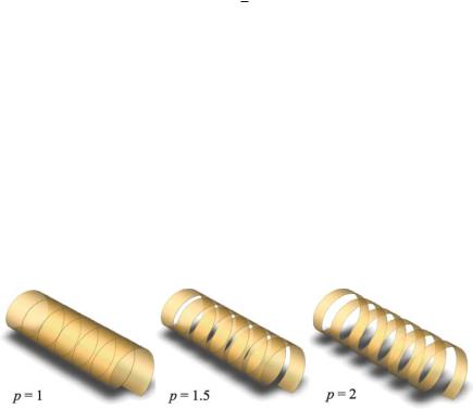
8 Three-Dimensional Fourier-Based Reconstruction Methods

today is available in Kalender ( ). There, the advantages and disadvantages of the corresponding interpolations are discussed in detail. This particularly also applies to devices with multi-line detectors and to methods with ECG triggering.

The speciﬁc scan protocol parameters of these methods will be brieﬂy discussed in the following paragraphs. Contrary to conventional CT, one has to consider the table speed vt as a function of the rotation frequency Trot of the sampling unit. This yields the table feed per rotation or the helical rise:

s = vt Trot .

( . )

If one includes the width or thickness of the X-ray fan d deﬁned by the collimator, then these parameters are usually combined to deﬁne the new scan protocol parameter pitch

s
p = d .	( . )

Here, this parameter is deﬁned for a system with a single detector array. Figure . illustrates the importance of the dimensionless pitch factor, which describes the table feed per rotation as a function of the slice collimation. Spiral acquisition trajectories with the pitch factors p = , p = . , and p = (from lef t to right) are shown. The table feed per rotation can obviously exceed the value of the slice thickness. Correspondingly, it has to be discussed whether or not the sampling theorem is violated in this situation.

In order to ensure that Shannon’s sampling theorem is not violated, overlapping slices have to be acquired for the three-dimensional reconstruction in conventional CT as already described in the previous section. This requirement does not necessarily have to be met in spiral CT scanners because – in principle – a sequence of arbitrarily ﬁne slices can be reconstructed from the spiral. Overlapping slices can therefore also be reconstructed retrospectively with this method. Figure . shows

Fig. . . Impact of the dimensionless pitch factor (table feed per rotation in units of the slice thickness) in spiral CT. Di erent pitch factors p (p = , p = . , and p = ) are illustrated from left to right. A pitch factor p reduces the acquisition time since a larger volume in

units of the slice thickness can be measured. The dose is obviously smaller for p = than for p =

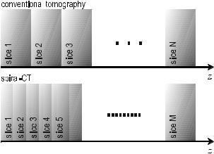
8.3 Spiral CT

Fig. . . A closer sequence of the images in the slice stack can be achieved by retrospective computation of the single slices with spiral CT (M % N). Therefore, staircase artifacts (cf. Sect. . . ) can be reduced within the three-dimensional representation (adapted from Kalender [ ])

schematically the number of slices in spiral CT compared with conventional CT. In this context, one should take into account the fact that the slices are getting closer to each other, but that, on the other hand, the thickness measured for each slice is still determined by the slice thickness selected with the collimator.

Nevertheless, there are still some restrictions concerning the selection of the pitch factor. The pitch factor, p, typically ranges from to . First of all, it should be clariﬁed why the method actually works for p = . As discussed above, the projection data are, according to ( . ), interpolated from neighboring real projections on the helix. If one assumes that a very small, δ-shaped object has to be measured, and if one further assumes that a theoretical slice thickness can be adjusted with the sampling unit having a δ-shaped sensitivity proﬁle, then the spiral CT method would not be successful at all. This is because the object would actually only be visible as a projection under a single angle. As a consequence, the Radon space for this object, approximated with the spiral CT interpolation scheme, would include inconsistent projection data, since no projection outside of the source orbit point at zr contains information of the δ-object.

However, in real systems one neither measures such small objects nor is the sampling unit provided with a δ-shaped sensitivity proﬁle. As long as a real object is located inside the proﬁle of one slice thickness while the patient table moves forward, the corresponding neighboring projections also provide information on this object. Therefore, an interpolation ﬁnally makes sense. But why does a pitch factor p actually work? In order to answer this question one may once again have a look at Fig. . . Due to the virtual supplementary helix, which has been shifted by , it is theoretically possible to track all object points for a su ciently long sampling period in the projections even with a pitch factor of up to p = . Data loss

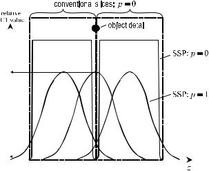
	8 Three-Dimensional Fourier-Based Reconstruction Methods

Fig. . . Advantage of spiral CT regarding imaging of small structures. The slice sensitivity proﬁles (SSP) for conventional and spiral CT are represented versus the axial z-axis. If very small details are located exactly on the border of the conventional slices, then the image intensity may be very small due to the steeply descending sensitivity proﬁle. In spiral CT, the maximum value of the slice sensitivity proﬁle is generally smaller, but, on the other hand, also softer and wider. As arbitrarily selected slice positions can be reconstructed retrospectively, the structure detail can subsequently be positioned exactly in the area of the maximum value of the spiral sensitivity proﬁle (adapted from Bushberg et al. [ ])

resulting in artifacts may arise for a pitch factor of p , especially if rather small structures are scanned. The pitch factors selected in practice range from < p < . .

Figure . schematically illustrates why conventional CT may under certain circumstances result in poorer image quality for small details than spiral CT. If a small structure is located exactly on the edge of two neighboring slices in a conventional tomogram with non-overlapping, densely arranged slices, then the intensity is equally distributed between the two slices even with a perfectly rectangular slice sensitivity proﬁle (SSP). Unfortunately, in practice, the SSP is only approximately rectangular so that the measured response of the system is further weakened as a function of the steepness of the proﬁle at the slice border.

On the other hand, a single-slice sensitivity proﬁle of each reconstructed slice is broader and ﬂatter in spiral CT than in conventional CT. This is due to the convolution of the conventional proﬁle with the table feed function. The higher the pitch factor the broader and ﬂatter the slice sensitivity proﬁle. Contrary to conventional tomography, in which the spatial location of the structure details in relation to the location of the slices is random and can only be corrected by a supplementary measurement with an additional radiation dose, it is possible to position the structure detail exactly in the center of the SSP in spiral CT. This can be achieved by computing the slices at any slice position retrospectively.

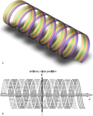
8.3 Spiral CT

It should be emphasized that the potential of the spiral CT method to compute arbitrarily dense overlapping slices does not mean that the spatial resolution in the axial direction can be increased arbitrarily. The axial resolution is always determined by the slice thickness given by the collimator (cf. Fig. . ). However, it is of course possible to reconstruct images every mm for a helix scanned with a fanbeam thickness of mm. But this does not ﬁnally result in a resolution of mm. In analogy to Bushberg et al. ( ), one should therefore distinguish between a -mm sampling pitch and -mm sampling aperture.

The demand for ever faster CT scanners has accelerated the development of multi-line detector arrays, which also run along a helical path. Figure . schemat-

Fig. . . a Helical orbits of a -line X-ray detector system. b Due to the concept of the inverse fan corresponding supplementary helices are shifted by for each real orbit. These are shown with dashed lines

8	Three-Dimensional Fourier-Based Reconstruction Methods
ically shows the corresponding paths of the actual detector lines as well as the cor-
responding supplementary helical paths for a -line detector array shifted by .
In this context, it is remarkable that only a single X-ray focus is used resulting in an
X-ray cone where mathematical analysis is computationally expensive, especially in
the case of a large cone aperture angle. However, good results can be achieved with
an approximate reconstruction method for small apertures in the axial direction
	. A discussion of the cone-beam reconstruction method will be the subject
of the following sections of this chapter.
(<	)
	Figure . exemplarily illustrates that the neighboring points used to interpo-
late the projection data for the slice at the axial position, zr, are even closer to each
other than in the geometrical situation shown in Fig. . . In order to evaluate this
fact with respect to image quality and radiation dose, one has to consider the num-
ber of lines M of the detector array related to the pitch factor so that
		p =	s
				.	( . )
			Md

Both the increased data acquisition speed and the reduction of radiation dose for pitch factors larger than one play a very important role in this context.

The main advantages of the spiral CT method can be summarized as listed in the following (Gay and Matthews ; Seeram ):

•Due to the continuous data acquisition synchronized with the table feed into the gantry it is possible to measure complete organs and larger volumes

on a short time scale. Shorter acquisition times result from both, a pitch factor, p , and, of course, the elimination of the table feed stop points that are characteristic of conventional CT.

•Due to the higher acquisition speed the number of artifacts associated with patient motion is reduced.

•Contrary to conventional CT, a complete data set can be acquired. Staircasing artifacts (cf. Sect. . . ) in the three-dimensional reconstruction can thus be eliminated.

•Slices can be reconstructed retrospectively at any axial position. Very small structures can also be visualized in this way.

However, it must be taken into account that the X-ray tube is subjected to an extreme load due to this continuous acquisition process. This particularly applies to the thermal stress. The reader of this book can ﬁnally evaluate the imaging quality of the spiral method by comparing the reconstructions shown in Figs. . and . . Figure . shows isotropic voxels with an edge length of . mm.

8.4 Exact 3D Reconstruction in Parallel-Beam Geometry

Fig. . . The success of the spiral CT method can be readily understood if again the vertebral phantom shown in Fig. . is used for evaluation. A uniform, i.e., the isotropic resolution of. mm has been computed retrospectively. Staircasing artifacts, as occurring in Fig. . , are considerably reduced here

8.4

Exact 3D Reconstruction in Parallel-Beam Geometry

The following sections will no longer deal with secondary reconstructions based on slice stacks, but rather with “true” three-dimensional reconstruction methods.

8.4.1

3D Radon Transform and the Fourier Slice Theorem

To deﬁne the Radon transform in the three-dimensional space corresponding to ( . ), one ﬁrst has to study how the D integration line deﬁned along the X-ray beam is now converted into a D surface. The projection integrals are thus converted into surface integrals. This means that a three-dimensional Radon value is a surface integral in the three-dimensional object space.

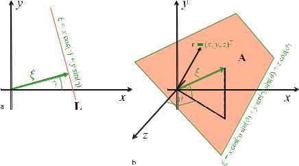
8 Three-Dimensional Fourier-Based Reconstruction Methods
In analogy to the deﬁnition of the unit vector
		=			( )
			cos		γ
	nξ		sin		(γ)			,	( . )
determining the corresponding projection angle γ for the two-dimensional recon-
struction method (cf. Fig. . a), the vector
	=	cos		γ	sin			ϑ
nξ	=	cos(		ϑ)		(		) "	( . )
nξ		sin (γ )sin					(ϑ )!		( . )
			(		)			#

suitably describes the analog “projection surface” in the three-dimensional space. Each surface A can in fact be unambiguously determined by a point in the Radon space if one interprets this point as the root point of the surface normal of A, the prolongation of which runs through the origin of the Radon space. Figure . b shows the surface A, which is the key element of the Radon transform in the threedimensional description. Analogous to the description in the two-dimensional space, the vector

ξx

ξ cos

sin

ξz

nξ

ξ cos(

ϑ)

(

) "

( . )

ξy

ξ sin

(γ )sin

(ϑ ) !

(

)

can be deﬁned, which unambiguously determines the Radon value.

Fig. . . a Geometrical description of the path of integration along a line L for the twodimensional reconstruction problem. b Description of an analog integration surface A for the three-dimensional reconstruction problem

8.4 Exact 3D Reconstruction in Parallel-Beam Geometry

A point r = (x, y, z)T is located in the plane A, if the inner product
ξ = (rT ċ nξ) = x cos(γ)sin(ϑ) + y sin(γ)sin(ϑ) + z cos(ϑ)	( . )

is constant. If A is a surface in the object space, then the sampling process can be described by

f (x, y, z) > δ(A) = ∫ f (r)δ(r − A)dr ( . )

i.e., in full analogy to ( . ) or

f > δ(A) = ∫ f (r)dr . ( . )

r A

Due to the sift property of the δ-distribution, ( . ) yields all points r of the object space located on the surface A. As the surface A is determined by (rTnξ) = ξ, the projection integral may again be expressed by

(

) =

(

)

((

) −

)

∫

nξ

∫

(x, y, z)δ(x cos(γ)sin(ϑ)

∫

∫ f

( . )

− − −

+ y sin(γ)sin(ϑ) + z cos(ϑ) − ξ)dx dy dz

=p(ξ)

i.e., in full analogy to ( . ). If the two-dimensional notation is consequently extended, the projection now changes with the two projection angles, γ and ϑ, so that

p = p(ξ, γ, ϑ) = pγ,ϑ (ξ) .

( . )

pγ,ϑ (ξ) is called the Radon transform of the three-dimensional object. One may write

f	(	) A R	• > ( ) =		γ,ϑ ( )
f		x, y, z ——— f δ A		p	ξ	( . )
or		pγ,ϑ (ξ) = R f (x, y, z) .
		pγ,ϑ (ξ) = R f (x, y, z) .				( . )

The three-dimensional Radon space consists of the surface integral values at the points (ξ, γ, ϑ) indicated by their spherical coordinates. The Fourier-slice theorem,

8 Three-Dimensional Fourier-Based Reconstruction Methods

which has already played a key role when we discussed the inversion of the Radon

transform in		Sect. . may also be formulated in three dimensions. For this pur-
pose, one	initially computes the Fourier transform of the Radon space again for all ξ
pose, one
of the corresponding projection angles γ and ϑ
				(								(		)
				(			) =−					(		)
			Pγ,ϑ			q		∫		pγ,ϑ			ξ		e− π i q ξ dξ ,			( . )
where the projection values pγ,ϑ ξ								in ( . ) result from the projection integral
extended into the two-			dimensional space (cf. ( . )),														i.e.,
extended into the two-					.		( )										i.e.,
					.												.
		Pγ,ϑ q	∫		-		∫ ∫			μ η, σ, ξ dσ dηB e− πiq ξ dξ
					.						(					)	.
					0												D	( . )
		( ) =− /− −							(					)			C	( . )
			=− − −						(					)
			∫ ∫ ∫					μ			η, σ, ξ				e− πiq ξ dξ dσ dη .

Figure . shows the relationship between the ﬁxed patient coordinate system and the rotating sampling system – consisting of the integration surface A – used for the description of the attenuation coe cients in the three-dimensional object space.

In the (x, y, z)-patient coordinate system, which still is a Cartesian but nevertheless a ﬁxed system that has been rotated by γ and ϑ and shif ted by the distanceξ

Fig. . . Relation between the ﬁxed (x, y, z) patient coordinate system and the coordinate system (ξ, η, σ) of the rotating surface A

8.4 Exact 3D Reconstruction in Parallel-Beam Geometry

one may write

(

)

(

)

(

))

) =− − −

Pγ,ϑ

∫ ∫ ∫

x, y, z

, σ

x, y, z

, ξ

x, y, z

e− πiq(rT ċnξ ) dx dy dz

(

)

=− − −

∫ ∫ ∫

x, y, z

e− πiq(rTċnξ ) dx dy dz .

( . )

Since both systems are of Cartesian nature, the integration element dξ dσ dη can be directly replaced by dx dy dz, because the corresponding Jacobian is equal to one.

On the other hand, the Cartesian formulation of the Fourier transform of the three-dimensional object in the ﬁxed (x, y, z)-patient coordinate system is determined by

(				(		)
(		) =− − −		(		)
F	u, v, w	∫ ∫ ∫	f		x, y, z		e− πi(xu+yv+zw) dx dydz .	( . )

Regarding the changes in the coordinate systems it should be recalled here that a point in the frequency domain with the spherical coordinates (q, γ, ϑ) is characterized by the Cartesian frequency coordinates

q cos

sin

= q sin

(γ )sin

(ϑ )

( . )

(

)

( )

w = q cos(

ϑ)

Therefore, the exponent in ( . ) may read

F(u, v, w) =

(

)

=− − −

∫

x, y, z

e− πi(x q cos(γ)sin(ϑ)+yq sin(γ)sin(ϑ)+zq cos(ϑ)) dx dy dz

(

)

=− − −

∫

x, y, z

e− πiq(x cos(γ)sin(ϑ)+y sin(γ)sin(ϑ)+z cos(ϑ))dx dy dz

(x, y, z)e− πiq(rT ċnξ) dx dy dz .

= ∫ ∫ ∫ f

( . )

− − −

( . )

8 Three-Dimensional Fourier-Based Reconstruction Methods

The integrand in the last line of ( . ) corresponds to the integrand of ( . ) so that the three-dimensional version of the Fourier-slice theorem can be summarized with

F(u(q, γ, ϑ), v(q, γ, ϑ), w(q, γ, ϑ))

= F(q cos(γ)sin(ϑ), q sin(γ)sin(ϑ), q cos(ϑ))

= Fspherical(q, γ, ϑ)

= Pγ,ϑ (q) .

8.4.2

Three-Dimensional Filtered Backprojection

Starting from the inverse three-dimensional Fourier transform of the object spectrum

	(			(		)
	(		) =− − −	(		)
f		x, y, z	∫ ∫ ∫	F	u, v, w		e πi(xu+yv+zw)du dv dw ,	( . )

spherical coordinates given by the system ( . ) are introduced here. As already indicated in the previous chapters, the inﬁnitesimal volume element du dv dw must be replaced by J dq dγ dϑ. T heJacobian J is here determined by

∂u

∂v

∂w

(

) =

∂q

∂u

∂v

∂w

∂ u, v, w

∂u

∂v

∂w

det

∂(q, γ, ϑ)

∂γ

( . )

(

)

(

)

H ∂ϑ

∂ϑ

∂ϑ H

(

)

sin

(

)

sin

(

)

cos

q sin ϑ .

cos

sin ϑ

( )

= −

( ) ( )

sin γ

sin

q cos

sin

) −

(

)

cos

(

)

q sin

(

)

(

q sin

q cos γ

cos

If one substitutes the new inﬁnitesimal volume element in spherical coordinates one ﬁnds the inverse Fourier transform

π π	F(q cos(γ)sin(ϑ), q sin(γ)sin(ϑ), q cos(ϑ)) ċ . . .
f (x, y, z) =ϑ =∫ γ =∫ q =∫

. . . ċ e πiq(x cos(γ)sin(ϑ)+y sin(γ)sin(ϑ)+z cos(ϑ))q sin(ϑ)dq dγ dϑ .

( . )

8.4 Exact 3D Reconstruction in Parallel-Beam Geometry

According to the Fourier slice theorem ( . ) it holds that
F(q cos(γ)sin(ϑ), q sin(γ)sin(ϑ), q cos (ϑ)) = Pγ,ϑ (q) ,		( . )
so that
π π	q sin(ϑ)Pγ,ϑ (q)
f (x, y, z) =ϑ =∫ γ =∫ q =∫	q sin(ϑ)Pγ,ϑ (q)	( . )

ċ e πiq(x cos(γ)sin(ϑ)+y sin(γ)sin(ϑ)+z cos(ϑ)) dq dγ dϑ .

For the inner integral, i.e., integration with respect to the frequency variable q, one may ﬁnd the abbreviated expression

f x, y, z

q Pγ,ϑ

q e πiq ξ dqBsin

dϑ dγ

(

∫

ϑ ∫

∫

( )

) =

∫

q Pγ,ϑ q

e πiqDξ dqBsin ϑ dϑ dγ

( . )

∫

( )

=−

π .

γ =∫ ϑ =∫

hγ,ϑ (ξ)sin(ϑ)dϑ dγ .

As mentioned above, for a ﬁxed point r = (x, y, z)T and ﬁxed projection angles γ and ϑ the projection surface A is determined by ξ. Obviously, in three dimensions,

	(			(		)
	(		) =−	(		)
hγ,ϑ		ξ	∫ q Pγ,ϑ		q		e πiq ξ dq	( . )

is the ﬁltered projection signal obtained by multiplying the Fourier transform of pγ,ϑ (ξ) with q in the frequency domain. The backprojection, i.e., smearing back the ﬁltered projection in a reverse direction, is given in the last line of ( . ).

8.4.3

Filtered Backprojection and Radon’s Solution

Similar to Sect. . it can also be shown here that the ﬁltered backprojection using hγ,ϑ (ξ) of ( . ) can be expressed in terms of the original solution by Johann Radon in (cf. introduction of Chap. ). Radon’s solution can be obtained even more easily than demonstrated in Sect. . because, thanks to the square of q in ( . ), the complicated Fourier transform of the absolute value function is not involved

	8 Three-Dimensional Fourier-Based Reconstruction Methods
	here. If one starts from ( . ) and takes the generalization of rule ( . ) for the
	inverse Fourier transform of the nth derivative of the spatial function f (x)

∫

(

i πu

)

n F

(

)

ei πux du

−

into account, then ( . ) reads

(

) = −

(

)

−

hγ,ϑ

∫

i πq

Pγ,ϑ

∂ pγ,ϑ

= −

∂ξ (

)

n
d dfx(nx) ,	( . )

(q)e πiq ξ dq

( . )

whereby the partial derivative indicates that the projection integral is a variable depending on ξ and the projection angles γ and ϑ. The reconstruction formula can then be derived from ( . ) into which ( . ) is substituted, so that

f x, y, z

q Pγ,ϑ q

e πiq ξ dqBsin

dϑ dγ

∫

(

) =

( )

=−

∂ pγ,ϑ ξ

∫

∂ξ ( )

sin

( . )

(

)

dϑ dγ

− ∂ pγ,ϑ

= −

∫

ϑ ∫

∂ξ (

)

sin

(

)

dϑ dγ .

Here, it has to be integrated over the entire unit sphere S, since the inﬁnitesimal surface element of the unit sphere is, as outlined in Fig. . ,

dS = sin(ϑ)dϑ dγ ;

( . )

thus, the Radon inversion equation can be given in the compact form

			∂ pγ,ϑ	ξ
f (x, y, z) = −		∫∫S	∂ξ (		)	dS.	( . )
	π

Because one integrates over all directions nξ a more formal expression, is given by

			∂ pγ,ϑ	ξ
f (x, y, z) = −		∫∫	∂ξ (		)	dnξ	( . )
	π

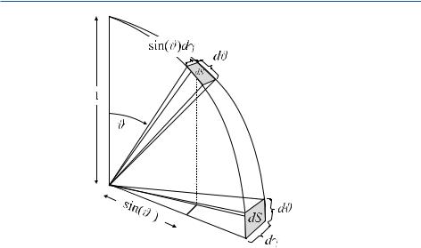
8.4 Exact 3D Reconstruction in Parallel-Beam Geometry

Fig. . . The inﬁnitesimal surface element dS of the unit sphere S depends on the polar angle ϑ with dS = sin(ϑ)dϑ dγ. Formally, the surface can be described by the inﬁnitesimal surface normal in the direction of nξ so that one has to integrate over all inﬁnitesimal directions dnξ

(Deans ; Natterer and Wübbeling ). Natterer and Wübbeling ( ) pointed out that the use of the three-dimensional inversion formula ( . ) must be seen as local tomography, because the calculation of f at the point (x, y, z)T only requires the surface integration in a rather close neighborhood of the point (x, y, z)T. More detailed considerations concerning the mathematics of local tomography are available in Ramm and Katsevich ( ).

8.4.4

Central Section Theorem

A variant of the Fourier slice theorem is called the central section theorem. This

modiﬁcation assumes that two-dimensional parallel projections pα,θ a, b						of the
three-dimensional object f		x, y, z		the underly-
	(		)	are available. Figure . outlines (	)
ing projection geometry.

In order to be able to describe the projection of the point r, assigned with the

attenuation value f r , along the straight lines deﬁned by the actual paths of the
three-dimensional space, it will be referred to here as the vec-
X-ray beams in the ( )
torial point slope form	r = ξ + ηnη
		( . )

of a straight line. The vector ξ is a distance vector, perpendicular to the detector normal nη , pointing to the projection line. This means that ξ lies within the detector

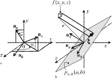
8 Three-Dimensional Fourier-Based Reconstruction Methods

Fig. . . a Orientation of the detector surface in the three-dimensional space using the detector surface normal nη , running parallel to the direction of the X-ray beams. The rotational degree of freedom around the detector normal is restricted by the unit vectors na and nb along the orthogonal principal axes of the detector. It is important that na is always positioned such that z = . b Projection of a point r = (x, y, z)T in the three-dimensional space along a line parallel to the detector surface normal nη (i.e., along the actual direction of the X-ray beams) onto the detector surface. Here, the orientation in space is determined by the unit vectors na and nb . pα,θ (a, b) denotes the projection values, i.e., the line integrals along the X-ray projection paths, which are measured at the point of intersection (a, b) on the detector plane

plane, i.e.,

such that the vector

ξ = ana + bnb ,

( . )

r ana

bnb

ηnη

( . )

describes in its parameterized

form the points on the projection line, which is per-

pendicular to the detector surface. The detector surface normal

cos

α sin

nη

(

)

(

)

( . )

sin(α)sin

(θ )

cos

(

)

is unambiguously determined by the spherical angles α and θ. Figure . a shows the position of the surface normal nη in the ﬁxed (x, y, z) coordinate system.

With the deﬁnition introduced above, the detector plane still has a rotational degree of freedom around the detector normal. Uniqueness is achieved by positioning

8.4 Exact 3D Reconstruction in Parallel-Beam Geometry

the detector vector na into the plane spanned by x and y, i.e., so that its z component is zero; thus,

sin

(

) "

( . )

−cos

(α )

This means, that

−

cos

cos θ

(

)

( )

( . )

− sin(α)cos(θ )

sin

(

)

is also uniquely determined.

Using the parametric representation ( . ) the X-ray projection can now be formulated as the line integral

pα,θ (a, b) =
pα,θ (a, b) =	∫ f (ana + bnb + ηnη)dη .	( . )

−

As illustrated in Fig. . b, pα,θ (a, b) is the measured X-ray projection value on the detector plane. Toft ( ) designates ( . ) as a hybrid or generalized Radon transform for lines in the three-dimensional space, although – strictly speaking – pα,θ (a, b) does not represent a Radon value (cf. Sect. . . ). Similar to the twodimensional situation, the hybrid Radon transform can be represented as a convolution with δ-distributions. This means

f (a na + b nb + η nη)

pα,θ (a, b) =η =∫− b

=∫− a =∫−

)

(

−

)

(

−

da db dη

( . )

f (ana

+ bnb + η nη)dη .

=η =∫−

The central section theorem – just like the Fourier slice theorem – actually relates the Fourier transform of the projection to the Fourier transform of subspaces of the three-dimensional space. The Fourier transform of pα,θ (a, b) can be expressed as

	(				(		)
	(		) =− −		(		)
Pα,θ		q, p	∫ ∫	pα,θ		a, b		e− πi(aq+b p)da db ,	( . )

where q and p are the frequency variables belonging to the spatial detector coordinates a and b respectively. Taking into account the deﬁnition of the hybrid Radon transform from ( . ), one may write

Pα,θ (q, p) =
Pα,θ (q, p) =	∫ ∫ ∫ f (ana + bnb + ηnη)e− πi(aq+b p) da db dη .	( . )

− − −

8 Three-Dimensional Fourier-Based Reconstruction Methods

As in the two-dimensional case, the expression has to be transformed to the ﬁxed patient coordinate system, i.e.,

	(a, b, η)T (x, y, z)T .						( . )
T his is feasible with a single rotation, since
	x	"	= (		a	"
r	= z	"	= (	na nb nη	) η	"	( . )
r	y	!		na nb nη	b	!	( . )
		#				#

(cf. ( . )) can be expressed by substituting ( . ), ( . ), and ( . ) into ( . ). This yields

sin

cos α

cos

sin

" =

−cos

( ) − ( ) ( )

( ) ( )

Qη

( . )

(α ) − sin(α)cos

(θ )

sin(α)sin

(θ )

sin

(

)

cos

(

)

η !

where Q is an orthogonal matrix, so that

Q− r

QTr

" =

(

)

(

)

( . )

−

sin

(

) −

cos

(

)

) "

= −cos (α )sin

sin

(

)

sin

(

cos

(

( ) (

)

sin

(

) (

)

cos

sin

! z

The Jacobian is thus J

and the inﬁnitesimal volume element is to be transformed

into

da db dη dx dy dz .

obey

( . )

According to ( . ) the three components of the vector (a, b, η)

b = −x cos(α) +

y cos

(

)

( . )

= −

x sin

(

)

(

) +

(

)

( ) (

) −

y sin

cos

z sin

( . )

cos θ

and

η = x cos(α)sin(θ) + y sin(α)sin(θ) + z cos(θ) .

( . )

Using the unit vectors ( . ) through ( . ), one may write in short

a = rT ċ na ,

b = rT ċ nb and η = rT ċ nη .

( . )

8.4 Exact 3D Reconstruction in Parallel-Beam Geometry

( . ) thus reads in the ﬁxed patient coordinate system

	(				(		)
Pα,θ		q, p	∫ ∫ ∫	f		x, y, z		e− πirT ċ(na q+nb p) dx dy dz .	( . )
			) =− − −
Obviously, the frequency vector				q = qna + pnb
				q = qna + pnb					( . )
in the three-dimensional frequency domain with the Cartesian representation ν										=
(u, v, w)T has the same orientation as										=
			ξ = ana + bnb ,						( . )

in the three-dimensional spatial domain with the Cartesian representation r = (x, y, z)T .

Figure . a shows how the distance vector ξ deﬁned in ( . ) can be identiﬁed with the Radon variable. The vector ξ is expressed with its spherical coordinates by the distance ξ and the angles γ and ϑ with respect to the ﬁxed (x, y, z) patient coordinate system, exactly as described above in Sect. . . . Figure . b illustrates the corresponding integration surface A of the Fourier slice theorem. This surface is perpendicular to the detector plane because the distance vector ξ lies in this very plane.

Fig. . . a The distance vector in ( . ) can be identiﬁed with the Radon coordinates ξ, which are determined by the distance ξ and the angles γ and ϑ in their spherical coordinates. The corresponding integration surface A is shown in b. Obviously, the surface A is perpendicular to the detector

8 Three-Dimensional Fourier-Based Reconstruction Methods

( . ) means that a

q, p

plane in the three-dimensional frequency domain

(with the Cartesian

coordinates u, v, and w

of the object f

x, y, z

to be recon-

(

)

dimensional Fourier transform P

structed, is identical with the two-

)

(

α),θ

q, p

of the

corresponding projection value or hybrid Radon transform p

α,θ a, b

on the

a, b

(

)

detector plane. The orientation of the detector plane

corresponds to the orientation

(

)

(

)

of the plane in the frequency domain, since the Fourier transform is rotationally

variant. In compact form, one may write

F pα,θ (a, b) = Pα,θ (q, p) = F(qna + pnb ) = F f (r) r =ξ = ana +bnb .

( . )

Figure . shows the central section theorem schematically. On the lower left side, the vertical projection of a single point f (x, y, z) onto an arbitrarily angulated detector plane can be seen in relation to a ﬁxed (x, y, z) patient coordinate system. As mentioned above, the plane of all line integrals perpendicular to the detector plane is the hybrid Radon transform pα,θ (a, b). A two-dimensional Fourier transform then yields Pα,θ (q, p). Due to the rotational variance of the Fourier transform, this plane is to be sorted into a ﬁxed (u, v, w) frequency space under the angulation of

Fig. . . Central section theorem. If all two-dimensional Fourier transforms (upper left) of three-dimensional parallel projections (lower left) are correctly sorted into the threedimensional Fourier space (upper right), then a three-dimensional inverse Fourier transform yields the original object (lower right)

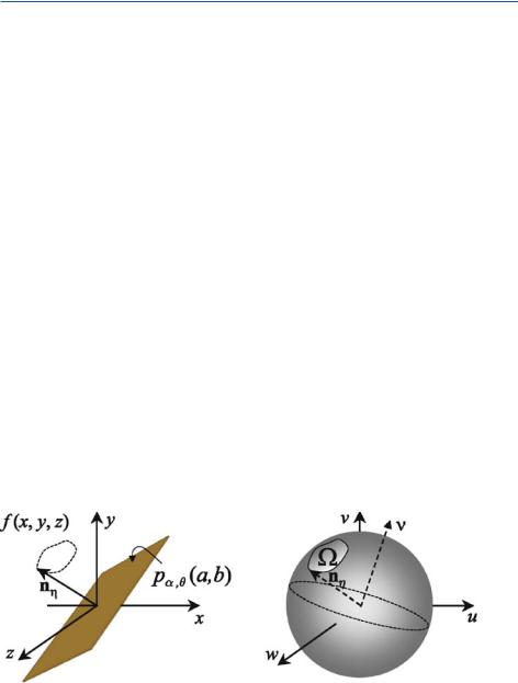
8.4 Exact 3D Reconstruction in Parallel-Beam Geometry

the measurement. If the projections have been measured for all angulations, then the object can ﬁnally be reconstructed by means of the inverse three-dimensional Fourier transform

	(				(		)
	(		) =− − −		(		)
f		x, y, z	∫ ∫ ∫	F		u, v, w		e πi(xu+yv+zw)du dv dw .	( . )

8.4.5

Orlov’s Sufficiency Condition

In the mid- s, Orlov ( ) had already answered the question as to how many parallel projections must be measured in order to reliably reconstruct the object – it must be noted that this question initially was answered in the ﬁeld of crystallography (cf. Orlov [ ]). According to ( . ) a set of parallel projections must be described by the hybrid Radon transform

(

)

(

)

pα,θ

) =−

=−

a, b

∫

dη

∫

ηnη

dη ,

( . )

where nη ; Ω S and Ω is the set of directions for which the parallel projections are actually measured. S again is the unit sphere of all directions and ξ is located in the projection plane described by the surface normal vector nη; therefore, obviously, (ξTnη) = . According to Orlov’s su ciency condition, F(ν), with ν = (u, v, w)T ; R , can be computed, if there is at least one projection direction nη ; Ω according to ( . ) for which (νTnη) = . Figure . shows a data acquisition situation in which the vector ν cannot be reconstructed.

Fig. . . Orlov’s su ciency condition. A requirement to be fulﬁlled by the measurement of parallel projections of all directions Ω (left) is that at least one direction must be perpendicular to the frequency vector ν. The whole frequency domain can actually be reconstructed if it is not possible to ﬁnd a great circle on the directional unit sphere S that does not intersect the area of the measured projections, Ω. The picture on the right side shows a great circle, which does not touch Ω. T he valuesF(ν) at the single frequency coordinate ν cannot be reconstructed with this measurement

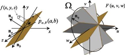
8 Three-Dimensional Fourier-Based Reconstruction Methods

Fig. . . The requirements stipulated in Orlov’s su ciency condition are met in the case of the continuous π rotation of the detector surface. This is due to the fact that the set of all directions, Ω, in which the parallel projections were measured, forms a great circle of the directional unit sphere S. Therefore, any other great circle on S intersects Ω

This condition ﬁnally implies that the object f (r) can only be reconstructed if the set Ω of the measured directions of the parallel projections is intersected by any great circle on the unit sphere, S. For Fig. . , illustrating the central section theorem, now the question can be answered as to whether the continuous rotation of the projection direction nη around the vector na is a complete measurement in terms of Orlov’s su ciency condition.

This is obviously the case, since the vector of the projection direction nη describes a great circle on the directional unit sphere S with this rotation. It thus is impossible to ﬁnd another great circle on S that does not intersect Ω. Due to Orlov’s su ciency condition, it is in fact obvious why the whole object cannot be reliably reconstructed with the tomosynthesis method described in Sect. . .

8.5

Exact 3D Reconstruction in Cone-Beam Geometry

The development step from parallel-beam to fan-beam tomography, which was discussed at the beginning of Chap. , resulted in two major advantages. First, the increase in acquisition speed that resulted from the fact that it was no longer necessary to stop for the parallel shift of the detector system while the sampling unit was rotating around the patient. The second advantage was better utilization of the tube heat capacity (cf. Sect. . . ). Using only a ﬁne pencil X-ray beam by pinhole collimation represents an enormous waste of the generated radiation. As the limited thermal capacity of the X-ray tubes to date still is a major technical problem, the measurements could be carried out much more e ectively by using fan-beam technology.

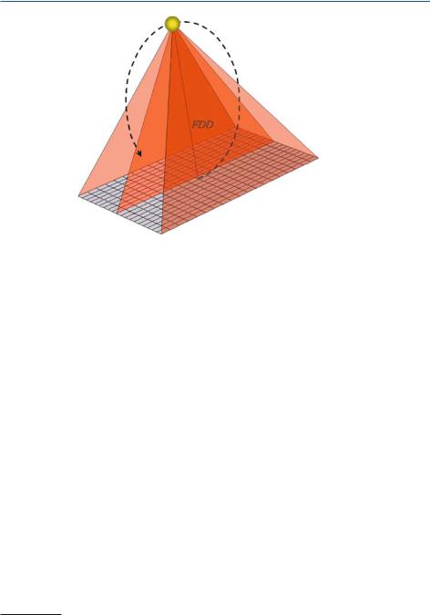
8.5 Exact 3D Reconstruction in Cone-Beam Geometry

Fig. . . Cone-beam illumination of a ﬂat-panel detector. Such arrangements are frequently used in technical applications such as material testing in micro-CT. Medical applications more frequently employ cylindrical detector arrays. However, there are already a few prototypes working with ﬂat-panel detectors in clinical applications

If one consequently follows the reasoning for fan-beam geometry, it seems to be useful not to employ only a collimated fan, but the entire cone beam generated by the X-ray source. This could technically not be realized for a long time, because

afast, high-quality, ﬂat-panel detector system was not available . However, twodimensional detector systems for CT scanners have recently been developed so that nowadays all manufacturers of CT scanners o er multi-slice CT (MSCT) systems.

Figure . schematically shows the cone-beam geometry of an imaging system with a planar detector (ﬂat-panel detector, cf. Sect. . . ). The planar detector geometry was ﬁrst of all applied for technical applications in micro-CT, since the required CCD chips were only available for this geometry. Anyway, Fig. . shows

aprototype of a so-called volume CT (VCT) developed by General Electric Medical Systems.

This type of CT scanner provides spatial resolutions, which were never attained before and were rather associated with micro-CTs. However, this improvement in image quality is achieved at the expense of demanding reconstruction mathemat-

ics, which will be described in the following sections. Figure . shows cone-beam projections over an angular interval of . The image actually shows the threedimensional projection data of a wasp, which was scanned using micro-CT. Con-

A major technical problem arises from the fact that the immense quantity of data must quickly be transferred from the rotating sampling unit to the processing system on the gantry or the scanner backend. These data must be transmitted via an interface with a large bandwidth. For this purpose optical slip-rings are used in modern scanners.

8 Three-Dimensional Fourier-Based Reconstruction Methods

Fig. . . Prototype of so-called volume CT in the GE research laboratories. A ﬂat-panel detector measuring approximately cm cm with a total number of , , pixels is arranged opposite to the X-ray tube on the sampling unit. This detector technology is described in Sect. . .

Fig. . . Three-dimensional sinogram of cone-beam micro-CT. The raw projection data of a wasp are shown over an angle interval of θ = [ , ]. The detector coordinates are denoted (a, b). Single projections are displayed in steps of

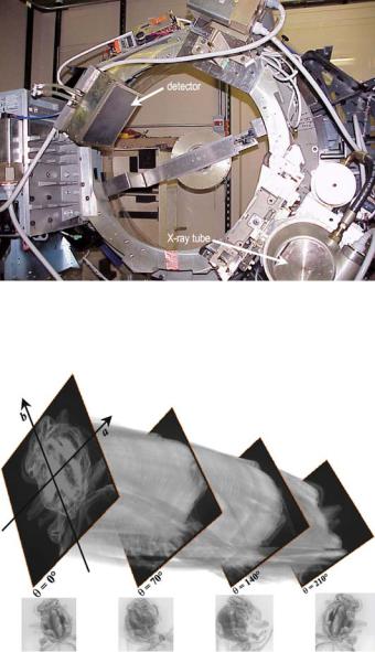
8.5 Exact 3D Reconstruction in Cone-Beam Geometry

trary to two-dimensional CT, the three-dimensional sinogram does not represent a Radon space. This problem will be discussed in detail in the following section.

8.5.1

Key Problem of Cone-Beam Geometry

As already shown in Fig. . , three-dimensional reconstruction methods require integration over two-dimensional surfaces to obtain the required data pγ,ϑ (ξ) in the Radon space (ξ, γ, ϑ).

If one has to deal with parallel-beam geometry, the surface integration can be split into two line integrals, the ﬁrst of which is along the X-ray beams

	T		(				(		)
	T		(		)U =−		(		)
Xp		μγ,ϑ		σ, ξ	∫	μ		η, σ, ξ		dη .	( . )

This equation is called the X-ray transform . Subsequently, the second integration is along the direction of the detector, σ:

(

( . )

) =−

pγ,ϑ

∫ Xp

μγ,ϑ

σ, ξ

dσ

(

)

=− −

∫ ∫

η, σ, ξ

dη dσ .

( . ) can readily be understood with Fig. . a.

Unfortunately, the simple separation of the surface integral into two line integrals makes it impossible to ﬁnd the required Radon values for the diverging X-ray beams, which almost always occur in practice.

If one ﬁrst integrates along the direction of the X-ray beams for the case illustrated in Fig. . b, i.e., if the X-ray transform, X ċ , is carried out in a ﬁrst step, then the adaptation to the geometrical situation requires the introduction of polar coordinates (r, φ). On the detector this yields the projection values

	T		(				(		)
	T		(		)U =−		(		)
Xc		μγ,ϑ		φ, ξ	∫	μ		r, φ, ξ		dr .	( . )

Indexing of Xċ with p or c denotes the X-ray parallelor cone-beam transform respectively.

8 Three-Dimensional Fourier-Based Reconstruction Methods

Fig. . . Di erence between parallel-beam and cone-beam geometry. a The parallel line integrals can easily be converted into a surface integral. b T his cannot so easily be done with cone-beam geometry

If these projection values are integrated along the detector, this results in the second integration

˜		c	Tμγ,ϑ (φ, ξ)U dφ
pγ,ϑ (ξ) =−π∫	X		Tμγ,ϑ (φ, ξ)U dφ					( . )
π				(		)
∫ ∫			μ		r, φ, ξ		dr dφ .
=−π −

To compare the result of parallel-beam geometry ( . ) with the result of conebeam geometry ( . ), ( . ) must also be transformed into the polar coordinates, i.e.,


	(				(			)
pγ,ϑ		ξ	∫ ∫	μ		η, σ, ξ				dη dσ
			) =− −								( . )
			π			(			)
			∫	μ			r, φ, ξ				r dr dφ ,
			=−π∫ −

where the Jacobian yields the variable r in the new inﬁnitesimal area element r drdφ.

8.5 Exact 3D Reconstruction in Cone-Beam Geometry

This means that the X-ray transforms

Xc Tμγ,ϑ (φ, ξ)U 8 Xp Tμγ,ϑ (σ, ξ)U ( . )

of the two geometries are not in line with each other; therefore, the data p˜γ,ϑ (ξ) do not represent the Radon values required for the reconstruction process in conebeam geometry. This means

˜	( . )
pγ,ϑ (ξ) 8 pγ,ϑ (ξ) .

8.5.2

Method of Grangeat

As shown in the previous section, there is no direct way to obtain the Radon transform in cone-beam systems. However, Grangeat ( ) has found a technique to compute a derivative of the Radon transform from the X-ray transform . One variation of the results will be discussed here. The main issues discussed in this section are adapted from a presentation by Jacobson ( ).

In a ﬁrst step, the Radon transform is di erentiated with respect to the direction of ξ, so that the expression

∂

(

) =

∂

(

)

pγ,ϑ

∫ ∫

r, φ, ξ

r dr dφ

( . )

∂ξ

−π −

can be obtained. Here, the order of the di erentiation and the integration may be changed, since one does not integrate over the radial Radon component ξ. T his results in

∂

(

∂

(

)

pγ,ϑ

∫ ∫

r, φ, ξ

r dr dφ .

( . )

∂ξ

) =−π −

∂ξ

To understand the meaning of the derivative ∂ ∂ξ, one has to study the geometrical conditions in the cone-beam projection. Figure . shows the corresponding three-dimensional geometry. In fact, one does not refer to a special source trajectory. Initially, the Radon data should be computed for an arbitrarily selected source detector situation from the projection data on the detector, which means from the cone-beam X-ray transform ( . ).

O denotes the detector origin and S denotes the X-ray source position. One now considers the use of a virtual detector situated in the iso-center of the measurement ﬁeld in order to simplify the geometrical approach. The results for other detector positions, especially those for situations found in practice, can then easily be derived from the intercept theorem.

The Radon sphere of the point S has the diameter FCD = eS − Oe and the detector surface is the tangential surface of the Radon sphere at the point O. T hat means that the vector S–O points in the direction of the detector normal.

A literature survey dealing with the three-dimensional cone-beam reconstruction is available in (Grangeat ).

8 Three-Dimensional Fourier-Based Reconstruction Methods

Fig. . . For an arbitrary trajectory of the X-ray source S, the derivative of the X-ray transform must be calculated from the detector data. For this purpose, a virtual detector is placed in the iso-center O of the measurement ﬁeld. An arbitrary fan of the X-ray cone-beam is shown shaded in red

As described in Sect. . . ,

ξ cos

sin

ξx

" =

ξz

nξ

ξ cos(

ϑ)

(

) "

( . )

ξy

ξ sin

(γ)sin(ϑ ) !

( )

unequivocally determines the Radon value pγ,ϑ

f x, y, z

, which is re-

This is due to the fact that the X-ray fan – i.e.,

quired for the reconstruction process.

( ) = R (

)

the integration surface through the point

r to be reconstructed – as described in

Sect. . . , is unambiguously determined by the vector ξ. ξ is perpendicular to this

X-ray fan, as illustrated with red color in Fig. . and it has its origin in O.

The foot-point of ξ on the X-ray fan and the points O and S form a rectangular

triangle on a great circle of the Radon sphere of S according to the theorem of Thales. T he central beam of the fan is tilted o the detector normal directionS–O by the angle κ. T he vectorr and the detector normal enclose the angle β.

The central beam of the fan, which is perpendicular to ξ, hits the detector at point R. The whole fan beam intersects the detector surface along the σ-axis. The intersection point P of the beam through the point r to be reconstructed can therefore be found on the σ-axis. The line connecting the detector origin O and point

In this consideration the vector r has its foot-point in the X-ray source.

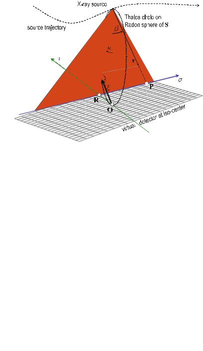
8.5 Exact 3D Reconstruction in Cone-Beam Geometry

R deﬁnes a radial detector τ-axis through O, which is always perpendicular to the X-ray fan-detector cutting line, σ. Figure . once again illustrates the described geometrical situation with a di erent perspective from that shown in Fig. . .

The derivative ∂ ∂ξ of the Radon transform proposed in ( . ) appears in the projection on the virtual ﬂat-panel detector as a radial derivative. As the detector data comprise the only physically measured reconstruction data basis, one thus ﬁrst has to study the consequences related to the variation of ξ with regard to the radial component ξ in ( . ) on the detector. The inﬁnitesimal change of the vector, ξ, by dξ results in a parallel shift of the σ-axis by dτ on the detector. However, the exact size of the inﬁnitesimal shift must be computed here . Figures . a and b illustrate the geometrical conditions in the X-ray fan plane (a) or perpendicular to this plane, respectively, i.e., in the plane (b) deﬁned by τ and S–O.

The point r to be reconstructed has the polar coordinates (r, φ) for a pre-deﬁned ﬁxed Radon vector ξ in the corresponding X-ray fan. As illustrated in Fig. . a the projection of the radius r onto the central beam of the X-ray fan is thus r cos(φ). This projection appears again in Fig. . b, which is a perpendicular view to the above ﬁgure.

Fig. . . A planar X-ray fan from the cone-beam is represented as a linear line of intersection along the σ-axis on the virtual detector in the iso-center O of the measuring ﬁeld. The projection of the Radon vector ξ on the detector deﬁnes a radial τ-axis through O, which is perpendicular to the σ-axis

As – by deﬁnition – the vector of ξ always ends on the Radon sphere, a change in the length with constant angles γ and ϑ results in the fact that the new vector points to the Radon data of other detector positions in space. This has to be accounted for in the case of the outline for an algorithmic implementation.

	8 Three-Dimensional Fourier-Based Reconstruction Methods

Fig. . . To compute the derivative of the Radon transform from the detector data, i.e., from the X-ray transform, the geometric situation inside a an arbitrary X-ray fan of the X-ray cone-beam and b the geometry within the surface that is perpendicular to this X-ray fan are illustrated

The variation dξ of ξ in the direction of the radial Radon coordinate ξ, which was proposed in the ﬁrst equation of this section, yields an inﬁnitesimally small vector, which can be shifted in parallel along a line R − S. This actually deﬁnes the inﬁnitesimal change of the fan tilt angle κ by dκ in the rectangular triangle deﬁned by the catheti dξ and r cos(φ) respectively. That means, the shorter the vector r, the larger the inﬁnitesimal angular change dκ related to dξ. This, in fact, determines the inﬁnitesimal parallel shift of the σ-axis by dτ.

Furthermore, Fig. . b also illustrates that

sin(dκ) = tan(dκ) =	dξ
	(	)
	r cos φ

or, because dκ is inﬁnitesimally small, that

dκ =	dξ
		.
	r cos(φ)

( . )

Additionally, Fig. . b shows that κ depends on ξ. Therefore, if a function v(κ(ξ)) is di erentiated with respect to ξ, the chain rule

∂v	=	∂v ∂κ	( . )

∂ξ		∂κ ∂ξ

8.5 Exact 3D Reconstruction in Cone-Beam Geometry

must be applied. The derivation of κ with respect to ξ can be replaced by an adaptation of ( . )

∂κ

∂ξ

so that

∂v = ∂ξ


=
		,
	r cos(φ)
∂v

∂κ r cos(φ) .

( . )

For convenience, the function v is deﬁned as the integrand in ( . ), i.e., the attenuation values weighted by the distance to the X-ray source

v = μ(r, φ, ξ) ċ r .

( . )

Then, ( . ) and ( . ) can be substituted into ( . ) to ﬁnd the expression

∂

(

∂

(

)

pγ,ϑ

∫ ∫

r, φ, ξ

dr dφ ,

( . )

∂κ cos(φ)

∂ξ

) =−π −

in which the order of integration and di erentiation can again be changed so that one ﬁnds

( ) =

(

) j

∂

−π

g−

∂

∂ξ pγ,ϑ ξ

∂κ ∫

cos

(

) g

∫ μ r, φ, ξ

( . )

dri dφ .

The integration along all X-ray beams yields the X-ray transform from ( . ) in the brackets of ( . ), i.e., we can ﬁnally ﬁnd the expression

∂			π
		∂
	pγ,ϑ (ξ) =		−π∫		Xc Tμγ,ϑ (φ, ξ)U dφ ,	( . )
∂ξ		∂κ		cos(φ)

which is the main result of Grangeat ( ).

In fact, ( . ) represents a fundamental relationship between the ﬁrst derivative of the Radon transform and the X-ray transform within cone-beam geometry. The key step is the substitution ( . ) because the right-hand side of ( . ) is relieved from the explicit r dependence. This is the only way to represent the integration over r – the bracketed term in ( . ) – as an X-ray transform, which has actually been measured.

However, the di erentiation with respect to the tilt angle κ is rather inconvenient, because in practice one actually has to deal with the principal axes a and b of the ﬂat-panel detector, which is shown in Fig. . . From Fig. . b, it can be read

8 Three-Dimensional Fourier-Based Reconstruction Methods

that

)

O tan

FCD tan κ

( . )

The di erentiation with

respect to the tilt angle κ yields

= e −

(

) =

(

dτ

FCD

( . )

dκ

cos

), one obtains

If one substitutes relationship ( . ) into ( .(

)

∂ξ pγ,ϑ (ξ) =	cos (κ) ∂τ		π	cos(φ)Xc Tμγ,ϑ (φ, τ(ξ))U dφ .
∂ξ pγ,ϑ (ξ) =	cos (κ) ∂τ		−π∫	cos(φ)Xc Tμγ,ϑ (φ, τ(ξ))U dφ .
∂	FCD	∂

For the second detector coordinate, it can be seen from Fig. . a that

σ = eS − Retan(φ) .

The di erentiation with respect to the fan angle φ yields

dσ = eS − Re dφ cos (φ) .

Furthermore, Fig. . a shows that

and thus

cos

(

) =

− e

− Pe

cos

dφ

(P) dσ

=ﬁnally,

can be substituted into ( . ) so that,

−

∂

FCD

Xc T

μγ,ϑ (σ, τ(ξ))U dσ

pγ,ϑ (ξ) =

−∫

∂ξ

cos

(

)

∂τ

−

( . )

can be found.

Figure . illustrates the meaning of the weighting introduced in ( . ). While integrating along the σ-axis of the detector, each detector point must be preweighted with its inverse distance to the X-ray source. This pre-weighting step can be expressed by β, i.e., the angle with respect to the detector normal direction S–O, so that

∂ξ pγ,ϑ (ξ) =	cos (κ) ∂τ			( . )
∂ξ pγ,ϑ (ξ) =	cos (κ) ∂τ		−∫ cos(β)Xc Tμγ,ϑ (σ, τ(ξ))U dσ .	( . )
∂		∂

In fact, the detector data can be pre-weighted for all detector positions before the integration is carried out. Of course, ( . ) only makes sense if the surfaces, deﬁned by the Radon coordinates ξ, actually contain the X-ray source. Otherwise, the distances eS − Pe are not deﬁned. This is the so-called Tuy–Smith condition, which will be discussed in detail in Sect. . . .

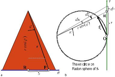
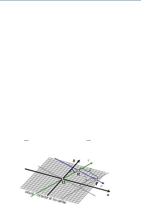
8.5 Exact 3D Reconstruction in Cone-Beam Geometry

8.5.3

Computation of the First Derivative on the Detector

( . ) means that it has to be integrated along the straight lines in the direction of the detector σ coordinate, namely, the detector values di erentiated in the direction of the detector τ coordinate. Here, the approach proposed by Grangeat will be used, which starts from the fact that the order of integration and di erentiation may be changed in ( . ). This leads to

	∂				∂		Tμγ,ϑ (σ, τ(ξ))U dσ ,
		pγ,ϑ (ξ) =		−∫		Xwc		( . )
where	∂ξ		cos (κ)		∂τ
	Xwc Tμγ,ϑ (σ, τ(ξ))U = cos(β)Xc Tμγ,ϑ (σ, τ(ξ))U							( . )

denotes the weighted X-ray projection.

Figure . illustrates that the (σ, τ) coordinate system is rotated by the angle δ with respect to the (a, b) principal detector axis system.

The radial di erentiation, which means the partial derivation of the weighted detector values in the direction of the τ coordinate, can be split into two terms. This can be done when using a description in components of the principal coordinate system, i.e.,

∂τ Xwc	Tμγ,ϑ (σ, τ(ξ))U = Ga (σ, τ)sin(δ) + Gb (σ, τ)cos(δ) ,	( . )
∂

where the partial derivation in the direction of the principal detector axes reads

Ga (σ, τ) = ∂a∂ Xwc Tμγ,ϑ (σ, τ(ξ))U and Gb (σ, τ) = ∂b∂ Xwc Tμγ,ϑ (σ, τ(ξ))U . ( . )

Fig. . . The (σ, τ) system is rotated by the angle δ with respect to the coordinate system of the detector principal axes a and b

8 Three-Dimensional Fourier-Based Reconstruction Methods

8.5.4

Reconstruction with the Derivative of the Radon Transform

( . ) provides an interesting relationship between the integration along radial derivatives on the ﬂat-panel detector and the ﬁrst derivative of the Radon transform with respect to the radial Radon coordinate. However, which advantage one may derive from this relationship with regard to object reconstruction remains to be clariﬁed. For this purpose, the geometrical situation will once again be studied in Fig. . .

The key idea of Grangeat is that ( . ) yields a value on the Radon sphere of the parallel projection, which is actually located at the point ξ = (ξ, γ, ϑ). However, this approach does not enable direct access to the Radon values, only to their ﬁrst radial derivative. These values are assembled on a meridian surface Vγ . T he polar orientation of Vγ just corresponds to the two Radon coordinates (ξ, ϑ).

All values ∂pγ,ϑ (ξ) ∂ξ are thus collected on di erent meridian surfaces, Vγ , which are inclined by the corresponding angle γ. For the complete object reconstruction

∂ pγ,ϑ

f (x, y, z) = −

∫∫S

∂ξ (

)

dS ,

( . )

Fig. . . The cone-beam projection does not provide a direct access to the Radon transform required for the reconstruction process. However, ( . ) yields a radially di erentiated value of the Radon transform on the corresponding point situated on the Radon sphere. These values are collected on a meridian surface Vγ , which includes the radial vector of the Radon point

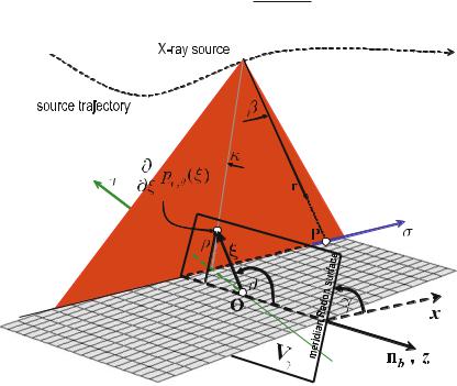
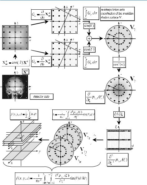
8.5 Exact 3D Reconstruction in Cone-Beam Geometry

Fig. . . Summary of the three-dimensional reconstruction method proposed by Pierre Grangeat

these values must once again be radially di erentiated and then azimuthally and polarly backprojected, as required by ( . ).

Figure . illustrates the individual reconstruction steps schematically. Starting with the cone-beam projection data on the ﬂat-panel detector (center left), the data are pre-weighted in a ﬁrst step. Next, the horizontal and vertical derivative may

8 Three-Dimensional Fourier-Based Reconstruction Methods
be considered separately. Thanks to the linearity of the integration operation in the
derivative images, one may now form the line integrals with respect to σ separately.
Both results are added after the sine and cosine weighting step have been car-
ried out. By interpolation, this value can be sorted into a virtual meridian detector
surface in the Radon space ξ				ξ, γ, ϑ . Another weighting step ﬁnally yields the
			transform.
radial derivative of the Radon= (				)
If another di erentiation is carried out once again in a radial ξ direction, one
actually ﬁnds the integrand that appears in the Radon inversion formula ( . ).
These values are schematically shown in the form of a Cartesian sinogram on the
lower right side of Fig. . .
The integration with respect to the inﬁnitesimal surface element dS introduced
in ( . ) corresponds to two consecutive backprojections: One in a polar direc-
tion, ϑ, i.e., inside the interpolated, meridian Radon surfaces, and the other in an
azimuthal direction γ, i.e., in parallel horizontal planes around the spatial z-axis.
Filtering of the data prior to backprojection, which is necessary for the recon-
struction process, is not readily visible within this method. However, the ﬁltering
step takes e ect in the penultimate step, because the Radon values, which have been
weighted with sin		ϑ and twice radially di erentiated, will be backprojected here.
This actually	corresponds exactly to the required ﬁltering step.
		( )

8.5.5

Central Section Theorem and Grangeat’s Solution

In this section the second reconstruction phase according to the Grangeat method is interpreted in terms of the central section theorem so that the backprojection instruction may better be understood. For this purpose, the parallel projection of the object to be reconstructed

	T		(				(		)
	T		(		)U =−		(		)
Xp		μγ,ϑ		σ, ξ	∫	μ		η, σ, ξ		dη ,	( . )

must be considered. Figure . outlines that this parallel projection is measured with vertical, perpendicular detector planes. nη denotes the detector surface normal vector and, as used in the previous sections, na and nb denote the principal detector axes. The detector surface normal vector determines the orientation of the ﬂat-panel detector, which is unequivocally described by the angle γ. The detector surface also represents the coordinates of the planes in the hybrid or generalized Radon space (cf. ( . )).

With this vertical deﬁnition, the unit vectors of the ﬂat-panel detector read

sin

cos γ

nη

( )

, na

( )

and nb

( . )

sin(γ)

−cos

(γ )

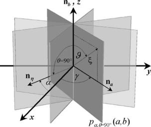
8.5 Exact 3D Reconstruction in Cone-Beam Geometry

Fig. . . Vertically arranged planar detector surfaces with the unit vectors pointing in direction of the principal detector axes na and nb . The surface normal of the detector is rotated by the angle α = − γ with respect to the x-axis of the ﬁxed patient coordinate system. The X-ray beams vertically pass through the corresponding ﬂat-panel detector surfaces. The measured projection values on the detector represent the values of the hybrid or generalized Radon transform

This constricted detector orientation is obviously the special case, θ = , of the deﬁnition of the unit vectors ( . ) through ( . ). The parallel projection Xp ċ thus also obeys the parameter representation of ( . ), i.e.,

pα (a, b) = pα,θ= (a, b) = Xp Tμγ,ϑ (σ, ξ)U = ∫ f (ana + bnb + ηnη)dη .

−

( . )

The central section theorem mentioned in Sect. . . ensures that the two-dimen- sional Fourier transform of the parallel projection is also available on a ﬂat plane in the three-dimensional Fourier space of the object. In this context, the orientation of the detector plane corresponds to the orientation of the ﬂat plane in the frequency domain, since the Fourier transform is rotationally variant. One may therefore write

F pα (a, b) = Pγ (q, p) = F(qna + pnb ) = F f (r) r =ξ = ana +bnb .

( . )

8 Three-Dimensional Fourier-Based Reconstruction Methods

The inverse Fourier transform of Pα

q, p

thus just yields the parallel projection

of the object to be

(

)

(

)U =

(

) =− −

μγ,ϑ

σ, ξ

pα

a, b

∫ ∫

qna

pnb

e πir ċ(qna +pnb ) dq dp .

( . )

Expressed with polar coordinates, the inverse two-dimensional Fourier transform ( . ) thus reads

(

)U =

(

) =

( )

−π∫ −

μγ,ϑ

σ, ξ

pα

a, b

∫

e πi(rTċν)

dν dϑ ,

( . )

where

q = qna , p = pnb and ν = q + p .

( . )

If, on the other hand, the Fourier-slice theorem described in Sect. . . is considered here, one may recall that

(

) =

(

)

) =− − −

x, y, z

u, v, w

∫ ∫ ∫

x, y, z

e− πiq(rTċnξ) dx dy dz

γ, ϑ

)

Fspherical(q,

(

)

πiq ξ

( . )

Pγ,ϑ

(

) =−

pγ,ϑ

e−

dξ

∫

= F R f (x, y, z) .

( . ) means that the one-dimensional radial Fourier transform of the three-di- mensional Radon transform is again available as a radial line in the three-dimen- sional Fourier transform of the object.

( . ) on the other hand ensures that the radial lines of the three-dimensional Fourier transform of the object located in the Fourier plane of the vertical ﬂat-panel detector correspond to the two-dimensional hybrid Radon transform. One thus ﬁnally ﬁnds

f x, y, z

pα a, b

(

x, y, z

)

( . )

so that theFobject(

to be)reconstructed= F (

obeys) = F

f (x, y, z) = F− F R f (x, y, z) .

( . )

Figure . summarizes ( . ) schematically.

8.5 Exact 3D Reconstruction in Cone-Beam Geometry

Fig. . . Illustration showing the relation worked out in ( . ). The one-dimensional, radial Fourier transform of surface integrals is identical with the radial line with the same orientation of the two-dimensional Fourier transform of the surface of the line integrals. Both frequency points are also available in the three-dimensional Fourier transform of the object

With this identity one may also write ( . ) as follows,

(

)U =

(

) =

(

)

−π∫ −

μγ,ϑ

σ, ξ

pα= −γ

a, b

∫ Pγ,ϑ

e πi(ξTċq)

dq dϑ .

( . )

As ( . ) is consistent with ( . ), it obviously describes the simple two-dimen- sional ﬁltered backprojection. This means that a parallel projection Xp ċ or the corresponding hybrid Radon transform of the object to be reconstructed respectively may be computed by a two-dimensional ﬁltered backprojection of the radial three-dimensional Radon values in vertical planes.

To understand the beneﬁt of ( . ), one should look once again at the threedimensional Radon inversion formula

			∂ pγ,ϑ	ξ
f (x, y, z) = −		∫∫	∂ξ (		)	dS	( . )
	π

8 Three-Dimensional Fourier-Based Reconstruction Methods

whereby the inﬁnitesimal surface element dS on the unit sphere S is determined by ( . ). Correspondingly, one may substitute the surface element to ﬁnd

∂ pγ,ϑ

(

x, y, z

) = −

γ ∫

∫π

∂ξ (

)

sin

(

)

dϑ dγ .

( . )

=−

The voxel

x, y, z

is reconstructed by the backprojection of the ﬁltered parallel

projection.(This

can be represented by

)

f (x, y, z) =

h PXp Tμγ,ϑ (σ, ξ)UQdγ ,

γ=∫

( . )

where

(

)UQ

(

)

(

)

( . )

=−π∫ −

μγ,ϑ

σ, ξ

∫

Pγ,ϑ

e πiξq q dq sin

dϑ

= −

π ∂ pγ,ϑ ξ

(

)

−

∂ξ ( ) sin

dϑ .

π∫

The method proposed by Grangeat is summarized in Scheme . . Artifacts related to practical implementation are discussed in Lee et al. ( ).

A comparison of ( . ) with ( . ) reveals that the ﬁltered parallel projection di ers from the simple parallel projection by a supplementary weighting factor sin(ϑ) and that it is ﬁltered with the linear frequency ramp q in the frequency domain. ( . ) and ( . ) correspond exactly to the two ﬁnal steps in Fig. . . ( . ) can be related to the parallel projection or the hybrid Radon transform pα (a, b) respectively, by using the central section theorem.

8.5.6

Direct 3D Fourier Reconstruction with the Cone-Beam Geometry

In Sect. . the method of direct inverse Radon transform based on the inverse Fourier transform for the two-dimensional case has been discussed. In theory, this approach is straightforward. However, problems related to the radially decreasing density of the sample points in the Fourier space of the Radon transform arise when this approach is implemented in practice. The linogram method (Jacobson ), which is described in Sect. . , was proposed as a countermeasure to these problems. It should be concisely discussed here that it is also possible to reconstruct successfully with a properly adapted linogram method in the case of three-dimensional cone-beam geometry.

8.5 Exact 3D Reconstruction in Cone-Beam Geometry

Scheme . Reconstruction with cone-beam geometry according to Grangeat

. Pre-weighting of the detector data

Xwc &μγ,ϑ (σ, τ(ξ))' = cos(β)Xc &μγ,ϑ (σ, τ(ξ))'

( . )

. Computation of partial derivatives in the direction of the principal ﬂat-panel de-

tector axes

∂

Ga (σ, τ) =

Xw &μγ,ϑ (σ, τ(ξ))'

and Gb (σ, τ) =

Xw &μγ,ϑ

(σ, τ(ξ))'

∂a

∂b

( . )

. Computation of line integrals on the detector and weighting of the results with the

factor cos

)

yields the radial derivative of the Radon transform, i.e.,

(

∂

) =

∫

(

)

(

) +

(

)

(

)

pγ,ϑ

σ, τ

sin

σ, τ

cos

dσ

( . )

cos

(κ)

∂ξ

(

−

. Interpolation of the data located on the Radon sphere given by ( . ) into vertical,

meridian Radon surfaces.

. Filtered backprojection within the vertical, meridian Radon surfaces, i.e.,

μγ,ϑ

(

σ, ξ

)', = −

∂ pγ,ϑ (ξ)

sin

(

)

dϑ .

( . )

−π∫

∂ξ

. Backprojection within horizontal planes by integration over the plane rotation angle, γ, i.e.,

f (x, y, z) =

*Xp &μγ,ϑ (σ, ξ)',dγ .

γ =∫

( . )

Sect. . . , equation

In F

(

q, γ, ϑ

)

q, γ, ϑ

)

, w

(

q, γ, ϑ

))

( . )

(

)

(

)

(

)

sin

)

, q sin

sin

, q cos

))

= Pγ,ϑ

cos γ

(

q, γ, ϑ

)

Fspherical

( )

summarized the applicability of the Fourier slice theorem to the three-dimensional reconstruction problem. In this context, it should be recalled here that the Fourier transform of the Radon transform is in line with the Fourier transform of the object on radial lines passing through the origin of the frequency domain. However, the previous sections have shown that direct access to the Radon transform pγ,ϑ (ξ) is not available within cone-beam geometry.

8 Three-Dimensional Fourier-Based Reconstruction Methods

The approach proposed by Grangeat only yields the radial derivative of the Radon transform, i.e., ∂pγ,ϑ (ξ) ∂ξ. But Grangeat also veriﬁed that the derivative is at least half the way to the ﬁltered backprojection. Unfortunately, within the direct Fourier-based reconstruction approach one does not need ﬁltered Radon data, but rather the native Radon transform pγ,ϑ (ξ). The following considerations will show how the expression ∂pγ,ϑ (ξ) ∂ξ can be integrated into the direct reconstruction approach.

In a ﬁrst step, the Fourier di erentiation property given in ( . ) has to be considered again. Due to this rule, the Fourier transform of the radial derivative of the Radon transform is given by

F M∂ξ pγ,ϑ (ξ)O = i πqPγ,ϑ (q) .				( . )
	∂
The Fourier transform of the Radon transform thus obeys
F Tpγ,ϑ (ξ)U = i πq F M ∂ξ pγ,ϑ (ξ)O .				( . )
			∂
The inverse Fourier transform then yields		∂ξ pγ,ϑ (ξ)O' .
pγ,ϑ (ξ) = F− &i πq F M		∂ξ pγ,ϑ (ξ)O' .		( . )
			∂

If one takes into account the Fourier result of the signum function mentioned inSect. . , i.e.,

sign(ξ) A———•		,	( . )
	iπq
the convolution theorem (cf. Sect. . )

pγ,ϑ (ξ) = F− &i πq F M ∂ξ∂ pγ,ϑ (ξ)O' = F− &i πq ' > F− MF M∂ξ∂ pγ,ϑ (ξ)OO

( . )

can be applied to ﬁnd the normal Radon transform by a convolution between the signum function and the radial derivative of the Radon transform, i.e.,

∂

pγ,ϑ (ξ) =

sign(ξ) >

pγ,ϑ

(ξ) .

( . )

∂ξ

With ( . ), it is found that

F Rγ,ϑ ξ(

)

(

) = F

f x, y, z

−

f x, y, z

( . )

= F−

TF T

( )UU

∂

−

= F

MF M

sign(ξ) >

pγ,ϑ (ξ)OO .

∂ξ

δ-distribution mentioned in

8.5 Exact 3D Reconstruction in Cone-Beam Geometry

However – similar to the two-dimensional case – the problem that the sampling density decreases with an increasing distance to the origin of the frequency domain still has to be solved. In Jacobson ( ), it has been shown that the linogram sampling method is also helpful here.

8.5.7

Exact Reconstruction using Filtered Backprojection

Kudo and Saito ( ) as well as Defrise and Clack (Defrise and Clack ; Clack and Defrise ) proposed an initial formulation for a ﬁltered backprojection based on the ideas proposed by Grangeat that have been described in the sections above. In order to illustrate the strategy within this approach the following section, similar to Yang and Horn ( ), is based on the general three-dimensional inverse Radon transform

			∂ pγ,ϑ	ξ
f (x, y, z) = −		∫∫S	∂ξ (		)	dnξ .	( . )
	π

Since a backprojection method should be established, a deﬁned, ﬁxed source location does not have to be assumed. Rather, this section deals with an X-ray source trajectory S(λ), parameterized by the continuous variable λ. This is necessary because – similar to all backprojection methods – each backprojection is carried out immediately after the projection has been acquired. Therefore, is not necessary to wait for the complete set of data of the Radon space before the reconstruction can take place. This principle is essentially the reason for the e ciency of backprojection methods.

Thus, it holds that

ξ S λ T n	,	( . )
since this expression describes the great= ( circle) ċ	ξon the Radon sphere for the source

position. Figure . illustrates the geometrical situation. To be able to reconstruct the point r, the contribution of the detector point P in the backprojection has to be found.

Taking into account the sifting property of the

Sect. . , one may write ( . ) as a convolution

dξidnξ ,

∂ pγ,ϑ

f r

∫∫

∫

δ ξ

nξ

( . )

∂ξ

( ) = −

g−

( )

(

−

ċ )

which even better indicates that the di erentiation takes place at all points r, which obey

ξ = rT ċ nξ .

( . )

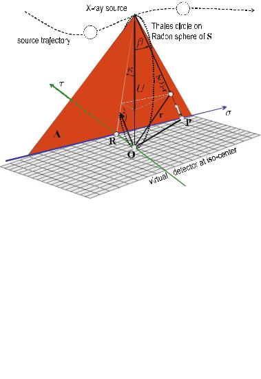
8 Three-Dimensional Fourier-Based Reconstruction Methods

Fig. . . Geometric situation of the cone-beam backprojection. The vector S(λ)has the same direction as the detector surface normal vector and the length of the distance between the detector and source -S − O-. The contribution of the detector value at the point P must be found in order to reconstruct the point r. A is the integration surface of the Radon transform. This plane is unequivocally determined by ξ = ξnξ

( . ) determines the integration surface A of the Radon transform shown in Fig. . . As the X-ray source must also be located in this plane, ( . ) must obviously be considered as a special case of ( . ).

Here, one actually does not want to consider a movement in the Radon space, but rather a movement of the X-ray source in the spatial domain for the backprojection. Therefore, it must be analyzed how the radial distance, ξ, in the Radon space is changed, in case the motion parameter λ of the X-ray source is varied. The amount of this change is determined by the variation of λ in ( . ), i.e.,

dξ	= SS (λ)T ċ nξS ,	( . )
dλ

where S (λ) is a tangential vector of the source trajectory at the orbit point S(λ). If one writes ( . ) as

dξ = SS (λ)T ċ nξS dλ ,

( . )

it is revealed that the radial sampling density along ξ depends on the trajectory direction. The factor can be understood as a compensation for the generally appearing irregular sampling of the trajectory.

To replace ξ and dξ, ( . ) and ( . ) are substituted into ( . ), which means the trajectory parameter λ of the X-ray source replaces the radial Radon variable.

8.5

Exact 3D Reconstruction in Cone-Beam Geometry

One ﬁnds

∂ pγ,ϑ

f r

∫∫

∫

ξ, λ

. . .

∂ξ

( ) = −

(

)9ξ=S(λ)

gΛ

ċnξ

( . )

. . . δ

(

)

nξ

−

nξ

)

(

λ, nξ

(

) ċ

nξ

In addition, the correction function

M(λ, nξ) =

( . )

n λ, nξ

has been introduced, which acts as a

compensation function for redundant meas-

(

)

urements of points in the Radon space. This is necessary because ( . ) may have

several solutions for arbitrary source trajectories. The function n λ, nξ

describes

the number of points of intersection of the source trajectory

S λ

(with

the integra-

)

tion surface A of the Radon transform. That is, a particular

Radon point p

γ,ϑ ξ, λ is

(

)

measured for an arbitrary source trajectory generally at n λ, n

source

positions,

(

)

or, in other words, the integration surface A is

illuminated at n λ, n

positions.

(

)

As the compensation function M λ, n

erent points in the

Radon space, it is used as a scaling(

ξ obviously varies for di (

)

function to prevent some Radon points from ex-

)

cessively contributing to the reconstruction of the object. As long as the su ciency

condition is fulﬁlled during data acquisition (cf.

Sects. . . and . . ), n

(

λ, n

ξ)

does not vanish.

An important issue in ( . ) is the integration in the domain of Λ, i.e., the

set of source trajectory points. In this way, the integration over the radial Radon

component is substituted here by a more convenient integration direction, required

for the backprojection procedure. The order of integration may be changed such

that

(

) = −

(

)

ξ=S(λ)Tċnξ

∫

∫∫

∂ pγ,ϑ

ξ, λ

. . .

∂ξ

( . )

)S ( ) ċ S

( ( ) − ) ċ (

. . . δ S λ r nξ M λ, nξ

λ nξ

dnξi dλ

is obtained to compute the backprojection instantaneously for each projection measurement.

According to Grangeat the ﬁrst-order derivative of the Radon transform is achieved by a di erentiation of the ﬂat-panel detector data. However, in ( . ) the second-order derivative is required. Therefore, it should be analyzed whether one of the two di erentiations may be replaced by an appropriate convolution. The required convolution kernel can be obtained by means of the Fourier representation of the ﬁrst derivative ( . ), which has frequently been used in the previous sections.

8 Three-Dimensional Fourier-Based Reconstruction Methods

The inverse formulation of ( . ) actually reads

∂

pγ,ϑ (ξ, λ) = F− Ti πqPγ,ϑ (q, λ)U ,

( . )

∂ξ

convolution theorem (cf.

Sect. . ) yields

so that the

∂

−

πq

−

q, λ

∂ξ

γ,ϑ (ξ, λ) = Fg ξ

i pγ,ϑ >ξ,Fλ

γ,ϑ (

( . )

where the convolution kernel

obviously reads

)

( ) >

(

) =−

∫

i πq ei πq ξ dq .

( . )

Substituting ( . ) in ( . ) one ﬁnds

(

−

)

∂p

ξ , λ

(

) −T )

. . . idλ .

∫∫ ∫ g

γ, ∂ξ

nξ

f r

ξ =−

(

)

∫ g

(

)

( ) = −

. . .

λ, nξ

nξ

dξ dnξ j

(j . )

Since ξ is the radial Radon coordinate, the convolution in ( . ) means that numerous parallel Radon integration surfaces (ξ , γ, ϑ) are needed from di erent source positions. This, however, jeopardizes the fundamental idea of backprojection, the advantage of which – compared with the Fourier method – is in fact the exclusive and self-contained treatment of each X-ray source position. For a particular λ, the integration surfaces described by ξ and ξ in the convolution in ( . ) cannot both contain the X-ray source.

On the other hand, for a particular λ on the Radon sphere of the X-ray source position S(λ), the theorem of Thales implies that ( . ) also applies to all other integration surface vectors that describe a great circle on this Radon sphere. For instance, one may also write

ξ = S(λ)T ċ nξ .

( . )

( . ) thus reads

					f		+
f	r	) = −				∫∫	∫
f	r			Λ		∫∫	∫
	(			Λ	g
			π		g	S	ξ =−
					g
				∫ g
					h

(

)

∂p ϑ

ξ , λ

. . . idλ .

(

−

)

γ, ∂ξ

(

) −

)

nξ

(

)

. . .

λ, nξ

nξ

dξ dnξ

. )

Figure . illustrates the geometrical situation of the new integration surface A . Now, the integration surface actually runs through the source as desired, but, unfortunately, the point r to be reconstructed is no longer included in the surface A .

8.5 Exact 3D Reconstruction in Cone-Beam Geometry

Fig. . . Geometrical situation of the cone-beam backprojection. If one varies the integration surface A by a variation of the integration surface vector ξ ξ on the great circle of the Radon sphere of S(λ), then the new integration surface A in fact still includes the X-ray source, but, unfortunately, does no longer include the point to be reconstructed

However, the convolution in ( . ) is a parallel displacement of the surface A . Fortunately, it can be shown that the undesired shift of the Radon variable ξ can be transformed into a shift of the radial detector variable, τ.

This transformation of the Radon variable into a detector variable is illustrated in Fig. . . From Fig. . a it can be deduced that

U
ξ − ξ = (τ − τ) cos(κ )FCD .	( . )

The inﬁnitesimal variation of the Radon variable must also be converted into an inﬁnitesimal variation of the detector variable. For this purpose, ( . ) has to be di erentiated, i.e.,

dξ	= cos(κ )	U
			.
dτ		FCD

Analyzing Fig. . b by means of the intercept theorem, the ratio

U	=	τ	cos	(	κ	)
FCD	=		τ	(		)

can be obtained so that the substitution reads

dξ = cos (κ )dτ .

( . )

8 Three-Dimensional Fourier-Based Reconstruction Methods

Fig. . . a Intercept theorems in the geometry of the cone-beam backprojection for the two cases ξ = S(λ)T ċnξ and ξ = S(λ)T ċnξ , as well as b for the inﬁnitesimal change of the radial Radon component ξ

( . ) and ( . ) are substituted into ( . ) so that one ﬁnds

(

−

)

(

)

τ =−

( ) = −

f ∫∫

∫

cos

FCD

. . .

(

)

( ( ) − ) ċ

f r

, λ

∫ g . . .

∂pγ,ϑ ξ

S λ r T nξ . . .

∂ξ

(

)

(

)

λ, nξ

nξ

cos

dτ dnξ

g . . .

i j j j j

jdλ . ( . ) j

j j k

The scaling property of the convolution kernel ( . ) with the argument of ( . ),

(

)FCD

=−

τ cos

∫ i πq ei πq τ cos(κ

)

dq ,

( . )

FCD

can be found by the substitution

= q cos(κ )

( . )

FCD

8.5 Exact 3D Reconstruction in Cone-Beam Geometry

The following can be obtained:

τ cos

∫ i πq ei πq τ dq

(

)FCD =

cos κ

FCD

−

FCD

(

)

g (τ)

and thus ﬁnally for ( . )

U cos (κ )

FCD

∂pγ,ϑ ξ

, λ

∫∫ ∫

g τ

. . .

∂ξ

)

S τ

(

−

)

(

=−

) = −

∫

. . .

(

. . .

(

) −

)

. . .

M λ, nξ

nξ cos

dτ dnξ

(

)S ( ) ċ

( )

i j j j j

jdλ . j

j j k

( . )

For a particular source position, ( . ) applies not only to the point ( . ), but also to all points on the great circle of the Radon sphere of S(λ); thus, one may substitute back ξ ξ.

The shift

yields

= S(λ)T ċ nξ

ξ = S(λ)T ċ nξ

( . )

∫

(

)

( ( T) − ) ċ

f ∫∫

∂ ∂pγ,ϑ ξ, λ

. . . idλ ,

f r

FCD

∂τ

∂ξ

S λ

r T

nξ

(

) ċ

(

)

. . .

λ, nξ

nξ

cos

( ) = −

dnξ j

( . )

where the convolution of the radial detector variable τ yields the di erentiation operator in analogy to the rules ( . ) through ( . ). The sift property of the δ- distribution may be replaced by changing the integration interval so that ( . ) becomes

( ) = −

FCD

∫∫

∂

∂pγ,ϑ

ξ, λ

M λ, nξ

∂ξ

i dλ .

f r

S λ r nξ

∂τ

(

)

( . )

π ∫

g( ( )− )

(

)

nξ

cos

(

dnξ j

To understand along which directions it must be integrated in the inner integral on the surface of the Radon sphere, Fig. . a also illustrates that the points obeying (S(λ) − r)T ċ nξ = are located on a circle on this surface.

All points of the circle contribute to the reconstruction of the object point r in the backprojections, since these are all fan surfaces inside the cone beam, which include the beam (S(λ) − r). All directions nξ perpendicular to this beam, deﬁne

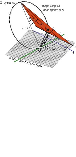
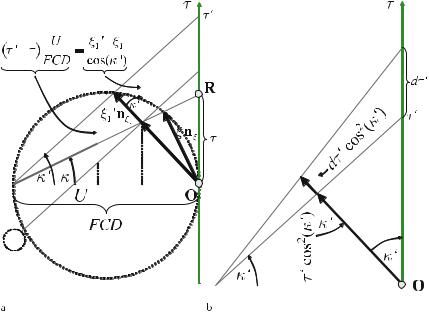
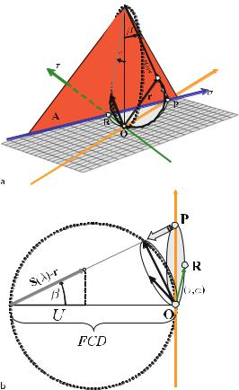
8 Three-Dimensional Fourier-Based Reconstruction Methods

Fig. . . The contributions to the detector backprojection point P are collected on a circle within the Radon sphere of S(λ). T heδ-distribution in equation ( . ) indicates that it must be integrated along the directional contributions on the Radon sphere, which obey (S(λ) − r)T ċ nξ = . These are all points (S(λ) − r).nξ located on a circle of the Radon sphere as illustrated in a. b shows that the integration over the directions nξ can be mapped on the detector by projection. The data at the position τ will be integrated on the detector over all angles α

a plane passing through the origin O and have the normal

S λ

r . T he section

of this plane with the Radon sphere of S λ

yields a circle

with a radius

( ( ) −

)

ξ)P nξP

( . )

(

That means, only the Radon values on this very circle contribute to the reconstruction. This applies to the reconstruction of all object points located on the beam passing through r. Moreover, this is in fact the characteristic feature of the backprojection. The ﬁltered projection values are “smeared” back in the direction of the original projection.

8.5 Exact 3D Reconstruction in Cone-Beam Geometry

Scheme . Exact reconstruction by backprojection within cone-beam geometry

. Computation of the radial derivative of the Radon transform according to

Scheme .

R (f (τ, α, λ)) = ∂ξ pγ,ϑ (ξ, λ)

∂

= cos

κ ∂τ

(

)

(

( ))

−

∂

(

)

∫ cos β X

μγ,ϑ σ, τ ξ

, λ dσ

( . )

. Weighting of the derivative of the Radon transform

) ċ

( )

R (

(

)) =

∂ξ

(

)

(

τ, α, λ

∂pγ,ϑ (ξ, λ)

λ, nξ

λ T

nξ

cos

( . )

. Di erentiation in the direction of the radial detector variable τ

Rw (f (τ, α, λ)) =

∂τ Rw(f (τ, α, λ))

( . )

∂

. Two-dimensional ﬁltered backprojection within the detector plane

hλ (a, b) =α =∫ Rw (f (τ, α, λ))dα

( . )

. Three-dimensional weighted backprojection

f (r) = −

Λ∫

FCD

hλ (a, b)dλ

( . )

In a last step, the appropriate ﬁlter operator still has to be found. In this context, Fig. . b illustrates that the projection of the circle located on the Radon sphere onto the detector yields an ellipse, the maximum diameter of which is eP − Oe. An arbitrary point ξnξ on the Radon sphere is projected onto the point τ located on the detector at the angle α described in the coordinate system of the detector. Therefore, in ( . ), the integration over the circle on the Radon sphere can be replaced with an integration over the corresponding ellipse on the detector.

Doing so, the expression

(

)

( ) = −

FCD

∂ ∂pγ,ϑ ξ, λ

( . )

∫

∂τ

∂ξ

M λ, nξ . . .

. . .

(

)

nξ

(

)

cos

dαi dλ

8 Three-Dimensional Fourier-Based Reconstruction Methods

can be found, where the ﬁrst derivative of the Radon transform must be replaced with the substitution term

∂ξ pγ,ϑ (ξ, λ) =	cos (κ) ∂τ			( . )
∂ξ pγ,ϑ (ξ, λ) =	cos (κ) ∂τ		−∫ cos(β)Xc Tμγ,ϑ (σ, τ(ξ)), λU dσ	( . )
∂		∂

found by Grangeat.

The inner integral in ( . ) represents a two-dimensional ﬁltered backprojection in the detector plane. The outer integral is a three-dimensional backprojection of the values from the inner integral, which have been weighted with the squared distance between the X-ray source and the point to be reconstructed. Scheme . summarizes the exact backprojection algorithm proposed by Defrise and Clack ( ).

8.6

Approximate 3D Reconstructions in Cone-Beam Geometry

The exact methods described in the previous section are based on a complete set of Radon data. However, as already mentioned in Sect. . . , complete Radon transforms can only be acquired if certain requirements with regard to the X-ray source trajectory are met. In the frequently used circular X-ray source orbit, one major problem is related to the fact that there are so-called shadow zones in which no Radon data are available.

8.6.1

Missing Data in the 3D Radon Space

In principle, the object can be reconstructed in the three-dimensional space. For this purpose, the methods used for the two-dimensional reconstruction must just be extended properly. In Sect. . it has already been veriﬁed that an exact reconstruction can be achieved with fan-beam geometry, if the coordinates are transformed accordingly. In Sect. . . the method proposed by Grangeat has been discussed, which contributes considerably to the solution of the inverse problem related to cone-beam geometry. However, in practice, a complete set of points in the Radon space is di cult to measure. Therefore, the corresponding problems of the frequently used circular acquisition protocol will be described in this section.

Figure . schematically illustrates the cone-beam geometry in an x–y section. For a circular trajectory of the X-ray source, located within this (x, y) plane, all object points of the plane can be exactly reconstructed in the spatial domain. If one considers a polar representation, the complete set of points in the Radon space belonging to a single point in the spatial domain is located on circles. The diameter of these circles connects the corresponding point in the spatial domain to the origin of

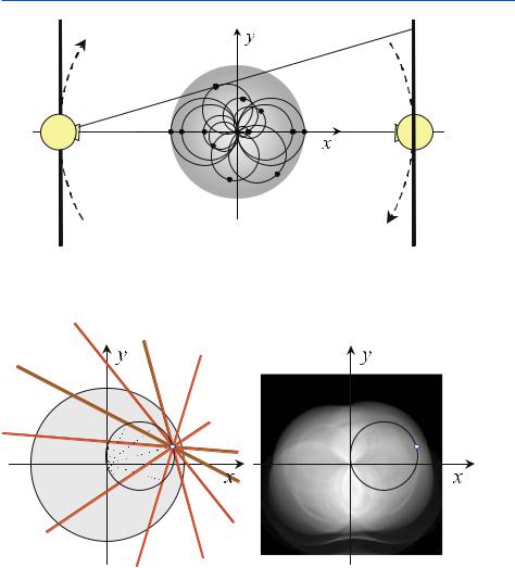
8.6 Approximate 3D Reconstructions in Cone-Beam Geometry

Fig. . . The circular trajectory of the X-ray source (dashed line) is located in the (x, y) plane. Thus, the sections of the integration surfaces in space just yield the integration lines known from the two-dimensional reconstruction problem

Fig. . . Left: As any point must have been illuminated from all directions (from up to ) in the reconstruction plane, circles in the Radon space according to the theorem of Thales can be found. Right: The Radon space is shown with its polar coordinates for a tomogram of the abdomen

the (x, y) plane. For a compact object in space, the Radon space is thus completely ﬁlled with those circles.

Figure . (left) illustrates that the circles in the polar representation of the Radon space can be geometrically derived with the theorem of Thales. Figure . (right) exemplarily shows the polar Radon space for an abdomen tomogram slice frequently used in the previous chapters. The corresponding circles are clearly visible.

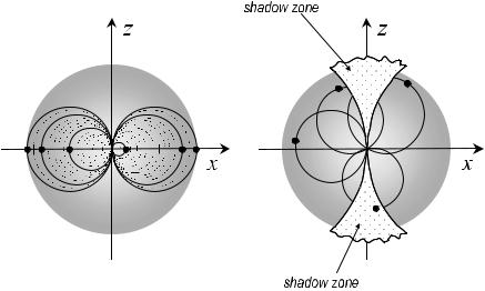
8 Three-Dimensional Fourier-Based Reconstruction Methods

Fig. . . Location of the practically available Radon values in the (x, z) plane. Left: As the set of Radon space values is complete for points in the (x, y) plane and the corresponding Radon values for each individual point are located on a spherical surface, the sections again result in circles. Right: Data are missing in the three-dimensional Radon space for points above and below the (x, y) plane. The zone in which data are missing is called the shadow zone

The Radon spheres can also be derived according to the theorem of Thales. They appear as rotational bodies of the circles rotating around their diameter lines between the origin at the reconstruction point in the spatial domain. Figure . (left) shows the location of the three-dimensional Radon values of points located on the x-axis that can be measured. The availability of the complete set of Radon values again refers to a single cyclic trajectory of the X-ray source in the (x, y) plane.

If there are points located outside the (x, y) plane, it will no longer be possible to measure all the points in the three-dimensional Radon space with this simple source trajectory. However, the following requirement must be met to exactly reconstruct the point. The Radon values of all points whose corresponding integration surfaces A intersect the object must be known for an exact reconstruction. According to the so-called Tuy–Smith su ciency condition (Tuy ) an exact reconstruction is possible if all surfaces intersecting the object intersect the trajectory of the X-ray source at least once.

The circles, however, have already been the result of the two-dimensional Radon space (cf. Sect. . ). Here, the three-dimensional reconstruction problem shall be solved. If, therefore, integration surfaces instead of integration lines are considered, the circles in the (x, y) plane can be found as sections of corresponding spherical surfaces in the three-dimensional Radon space.

Since the X-ray source must be located in the surface A in order to measure its integral, this also makes sense from an intuitive point of view. Points in the Radon

8.6 Approximate 3D Reconstructions in Cone-Beam Geometry

space, which cannot be measured with the planar cyclic source trajectory, are located in the so-called shadow zone illustrated in Fig. . (right).

Figure . once again shows points that comply with the Tuy–Smith condition. Such points are of course located in the (x, y) plane. The conical X-ray beam illuminates a spherical object. If only those points located within the (x, y) plane have a complete set of Radon data, then the sphere cannot be exactly reconstructed with this measurement. Figure . shows some outermost points with a complete set of Radon values on the front hemisphere of the spherical object.

Figure . schematically shows the formation of a shadow zone. If points r = (x, y, z)T are located outside the (x, y) plane, it will no longer be possible to measure the projection pγ,ϑ (ξ) for all projection angles γ, ϑ and distances from the origin ξ due to obvious geometrical restrictions.

Within the shadow zone the X-ray source is in fact located underneath the horizon of the integration surface A. This is exactly the Tuy–Smith su ciency condition. Those points that can, in principle, be measured with geometrical parameters result within a torus. Figure . shows the ﬁlling of the Radon space for the cyclic source orbit in the plane. The resulting torus includes all points that can theoretically be measured in the Radon space. But, in practice, it is not possible to measure all the points of the Radon space inside this torus as a detector has a ﬁnite size.

Source orbits meeting the requirements stipulated by Tuy–Smith are shown in Fig. . . Figure . a provides a comparison with the cyclic, planar trajectory of the X-ray source, which is responsible for the above-mentioned shadow zone in the Radon space. Figure . b shows one of the possibilities of ﬁlling up the shadow zone with Radon data. This is possible by using two circular X-ray source trajec-

Fig. . . In cone-beam geometry those object points for which the Radon space is complete are located within the plane deﬁned by the X-ray source trajectory. For a spherical object this applies to all those points within the circle that results from a section of the trajectory plane through the sphere. Some outermost points with a complete set of Radon values are exemplarily shown on the front hemisphere of the spherical object

8 Three-Dimensional Fourier-Based Reconstruction Methods

Fig. . . There are points in the Radon space, of the cyclic source orbit in a plane, for which the necessary integration over the surface cannot be carried out. The points assigned in the spatial domain may then not be correctly reconstructed. The Radon values for which the integration surface does not intersect the X-ray source orbit are missing. The missing zone in the Radon space is again the shadow zone

Fig. . . In the Radon space of the cyclic source orbit those points that can theoretically be measured are located within a torus. Nevertheless, it is in fact not possible to measure all theoretically available points of the Radon space with a detector of ﬁnite size

tories located in planes that are parallel to each other and connected with a linear trajectory . Figure . c shows two source trajectories that are perpendicular to each other and also circular. The requirements stipulated by Tuy–Smith are also met here. However, it can readily be understood that this option is excluded in medical

The linear movement is performed anyway, because a planning overview is always measured prior to the tomographic data acquisition (cf. Sect. . ).

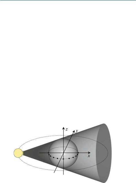
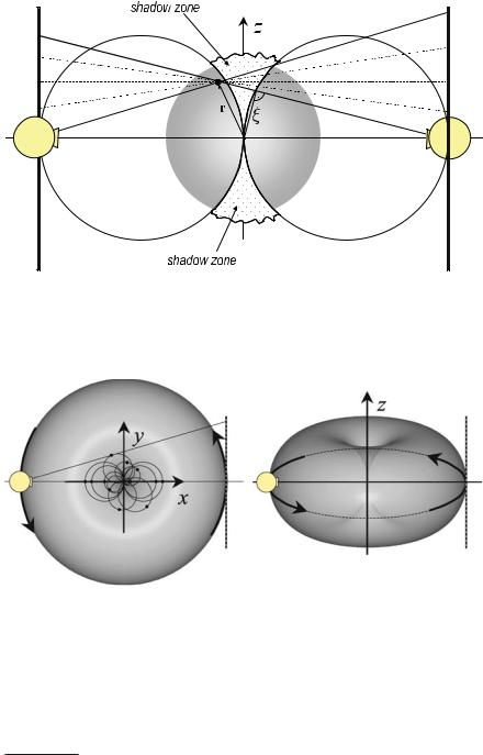
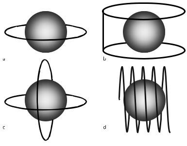
8.6 Approximate 3D Reconstructions in Cone-Beam Geometry

Fig. . a–d. Orbits of the cone-beam X-ray source sampling the Radon space. Apart from the simple cyclic path shown in a, all other trajectories meet the requirements stipulated in the su ciency condition of Tuy–Smith. The cone-beam helical path is used in modern medical CT scanners today

applications, because the patient is located in the source path. Practical applications typically use cone-beam helical paths scanning the Radon space with a continuous movement. This path is outlined in Fig. . d. The trajectories shown in this ﬁgure are not the only ones being tested at present. Another approach with a central circular orbit and a single supplementary line is proposed by Lin ( ). All these approaches are attempts to ﬁll up the shadow zone of the Radon space as e ectively as possible.

8.6.2

FDK Cone-Beam Reconstruction for Planar Detectors

The methods of three-dimensional reconstruction described in Sect. . are based on the assumption that a complete set of Radon data is available. However, as discussed in the previous section, the requirements stipulated in the Tuy–Smith su - ciency condition are not met for any source trajectory. This is particularly the case for the popular circular X-ray trajectory in cone-beam geometry used in many technical applications, where a complete set of Radon data is therefore not available. However, approximation methods that can also deal with incomplete Radon data of this type are available.

The most frequently used method is the reconstruction approach proposed by Feldkamp, Davis, and Kress (FDK) in (Feldkamp et al. ), which is

8 Three-Dimensional Fourier-Based Reconstruction Methods

a derivative-free method. The so-called FDK cone-beam reconstruction is an approximation of the exact reconstruction problem developed for technical investigations . As planar detectors are used for these applications, Feldkamp, Davis, and Kress (Feldkamp et al. ) initially presented their approximation for this geometry. Figure . shows the geometry of the sampling unit schematically.

The cone-beam geometry with the planar detector arrangement has a cone angle κa at the fan angle, ψ, which is deﬁned by the expression

b	.
κa = arctan 6a + FCD	.	( . )

With this deﬁnition, it is clear that the cone angle varies along the individual rows (i.e. b = const.) of the planar detector. Despite this, the geometry of the planar detector ﬁeld is well adapted to the backprojection described above. This is due to the fact that the integration over the surfaces can be realized by integrations along straight lines on the detector.

Figure . shows a tilted fan beam of the X-ray cone beam, which intersects the detector on a line with constant b. This geometry will have to apply to all fan beams inside the cone beam. The contribution of the point (a, b) to the backprojection has to be computed.

The FDK reconstruction is based on the assumption that every fan-shaped surface in the cone beam deﬁned by a detector line b and the X-ray source location must be treated independently, as if dealing with a two-dimensional fan projection as described in Sect. . . . Figure . shows such a surface. Just because a straight line on the detector is assigned to an integration surface (red-shaded fan), with planar detector geometry, one may access the detector independently line by line for the FDK reconstruction.

If the cone-beam projection system is considered under a ﬁxed projection angle θ, then the mathematical treatment of the individual projection fans within the X-ray cone does not di er from the treatment of the fans in Sect. . . . Due to the angulation κa of the fan o the (x, y) plane, only distances must be adapted appropriately. It is therefore obvious that ( . ) has to be slightly extended to take into account the new distances within the tilted fan. The ﬁltered backprojection may then be carried out exactly with reference to a single, ﬁxed angle under which the projection is considered. Similar to Sect. . . a virtual detector is placed in the iso-center of the system. The geometrical projection situation can then be more easily formulated mathematically.

The results can be applied to the real detector surface by means of the intercept theorem. Figure . illustrates that the projection of a point r = (x, y, z)T in the X-ray cone onto the detector position (a, b) depends on the fan angle ψ via

a = FCD tan(ψ)

( . )

Feldkamp, Davis, and Kress developed this method in the research laboratories of the Ford Motors for material testing.

8.6 Approximate 3D Reconstructions in Cone-Beam Geometry

Fig. . . Cone-beam illumination of a ﬂat-panel detector. The X-ray source rotates on a circle with radius FCD (focus center distance). A virtual detector is positioned in the iso-center of the rotation of the sampling unit. ϕθ (a, b) are the measured (virtual) projection values. The angle θ between the y-axis and the central beam of the cone – or the x-axis and the a-axis – deﬁnes the projection angle of the system

Fig. . . Cone-beam illumination of a ﬂat-panel detector. Only fans are considered within the cone that intersect the detector on a straight line with constant b. The contribution of the detector value at the detector point (a, b) to the backprojection will have to be determined

8 Three-Dimensional Fourier-Based Reconstruction Methods

and the cone angle κa via

b = G

tan(κa) .

FCD +a

( . )

In this system, the

a, b detector surface rotates about the z-axis describing the

axial direction of

the ﬁxed patient coordinate system.

(

)

The small principal axis of the detector, b, has been assigned to the negative

z direction to ensure that the detector system remains a right-handed system. The

angle θ between the y-axis and the central beam of the cone – or the x-axis and

the a-axis respectively – deﬁnes the projection angle of the system. FCD once again

stands for the focus center distance. It is possible to deﬁne a new coordinate system,

where the unit vectors nσ , nη, and nξ are shown in Fig. . . Here, nσ points into the

direction of the long a-axis of the detector. nσ is rotated by the angle θ with respect

to the x-axis. This is done by means of the orthogonal matrix Σ. nη points in the

direction of the source along the central beam of the angulated fan and nξ

nσ

nη

in the direction of the fan surface normal of A. nξ is thus rotated about

the angle

κ = arctan

( . )

FCD

with respect to the z-axis, which means about the nσ -axis. This corresponds to a multiplication with the orthogonal matrix Ξ.

Fig. . . Geometrical situation using a virtual detector in the iso-center of the sampling unit. As a straight line on the detector is assigned to an integration surface (transparent plane) for ﬂat-panel detector geometry, the detector values can be accessed line by line in the case of the Feldkamp, Davis, and Kress (FDK) reconstruction. The unit vectors nσ , nη , and nξ deﬁne the fan surface considered, where nξ = nσ nη is the surface normal of A

8.6 Approximate 3D Reconstructions in Cone-Beam Geometry

Finally, the transformation

s	!	ρ Ξ Σr b	Ξ	Σ	y !		!!		( . )
r		= = ( − ) =			x	"		""
t	"	= = ( − ) =		z		"	+ b	""
	#					#		##

is obtained. The point to be reconstructed may thus be expressed with the new coordinates as

cos

sin

sin(

θ)

cos(

θ) ! y

κ )

cos

sin

" =

−

sin(

cos(

κ )

−

( )

" z

" + b

(

)

(

)

x cos

y sin

κ )

) "

sin(

cos(

κ )

−

( z) +b

(

cos

)

sin

)

x sin( θ) +

y cos(

θ)

−

(

= −

(

)

(

x cos

(

y sin

) + (

)

(

) +y cos

)

cos

(

sin

x sin

θ cos κ

cos

)

(

) +

(

)

(

x sin

(

)

sin

(

) −

(

)

sin

) + (

cos

) #

On the other hand, one ﬁnds points ρ in the original coordinate system by

r = ΣT ΞTρ − b ,

( . )

which means

sin

( )

(

)

cos

(

) −cos

(κ

)

" t

− b

( . a)

sin

(θ ) −cos

(θ

)

sin

cos

sin

(

)

(

)

(

)

( )

(

)

s cos

) −

t sin

( . b)

sin

(θ ) −cos

(θ

)

s sin

(

) +

t cos

(

) −

r sin (θ ) −cos(θ)(s cos(κ ) − t sin(κ ))

( . c)

r cos

s cos

t sin

(

)s+sin

(

( )( t cos( κ ) −

(

)) "

) +

(

) −

As only those points inside the integration surface A are of interest, which are spanned by nσ and nη , t = might be assumed here. Thus, only the fan beam plane

8 Three-Dimensional Fourier-Based Reconstruction Methods

has to be dealt with in which

r cos

s sin

(

cos

(

)

( ) +

r sin

(θ ) −s cos(θ)cos(κ )

s sin

(

) −

FCD#

(

r cos

) −

FCD

s sin

FCD

( . )

( ) +

( )

s cos

r sin

FCD

−

(

)

FCD

(

system.

corresponding point

x, y, z

)

assigns to each point

r, s

the

#T patient coordinate

In full analogy with the approach described in

Sect. . . , an appropriate trans-

formation to parallel-beam geometry has to be

found to reconstruct the point ρ

lying in the fan angulated about the angle κ . In this way, the virtual parallel projection pγ (ζ) under the projection angle γ at the detector position ζ can be calculated within this fan of the X-ray cone beam. The virtual ζ coordinate is shown in Figs. . and . by a dashed line. It runs through the origin, which has been shifted by b with respect to the detector coordinate system within the fan, and forms a right angle with the X-ray beam through point ρ.

The relation with the fan-beam coordinates can be – in analogy to ( . ) and

( . ) – expressed by

FCD

a cos

( . )

(

) =

+a+

+ b

and

6FCD

γ = θb + φ =

θb + arctan

( . )

FCD +b

The new coordinates are illustrated in Fig. . . Thus, the three-dimensional conebeam reconstruction problem is reduced to a problem of two-dimensional fanbeam geometry (cf. Fig. . ). One may therefore use the equations of the ﬁltered backprojection in the fan-beam plane that have already been introduced inSect. . . . With the new coordinate notations ( . ) now reads

(

) =

(

)

(

−

)

r, s

∫

∫ pγ

ρT

nζ

dζ! dγ ,

( . )

whereby the relation with the x, y, and z components of r must be realized later by ( . ). The same strategy that has been followed in the previous chapter applies here. The fan-beam coordinates have to be substituted by parallel-beam coordin-

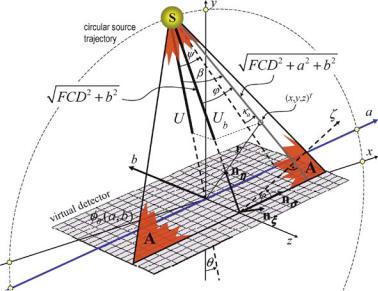
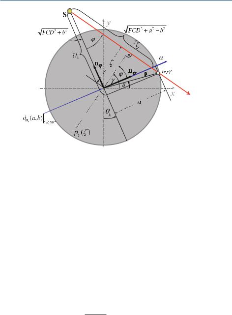
8.6 Approximate 3D Reconstructions in Cone-Beam Geometry

Fig. . . Geometry within the angulated fan-beam plane illustrated in Fig. . . The projection of the ﬁxed patient coordinate system is used as a reference system. This is an approximation only, due to the projective geometry. Nevertheless, this system can be used, because just a ﬁxed reference system is needed in which the sampling unit rotates about the nξ unit vector. As the backprojection is actually carried out over the full angle interval θb = [ , π] the result does not depend on the precise starting angle. The angles φ, δ, and γ are only required as relative angles with respect to the angle θb and do not refer to the actual (x, y, z) coordinate system. The relation between θb and θ will be explained later

ates. To do so, the coordinate transformation
(ζ, γ) (a, θb )	( . )

has to be carried out. As already shown in several other cases, the new inﬁnitesimal integration element must be scaled by the Jacobian. This means that the area element dζ dγ is determined in the new coordinates by J da dθb , where J is given by

∂ζ

∂γ

(

) =

∂θb

∂ ζ, γ

∂a

det

∂

(a, θb)

∂ζ

∂γ

( . )

8 Three-Dimensional Fourier-Based Reconstruction Methods

If the transformation equations ( . ) and ( . ) are directly substituted in

( . ) one ﬁnds

FCD

∂

∂a+

∂

θb

∂a

arctan

∂

FCD

(

)

6FCD

∂

θb

∂θb

( . )

FCD

b !

= 6FCD

( )

FCD

cos

φ .

inﬁnitesimal#

area element must be replaced by

This means that the+

FCD

dζ dγ

da dθb .

( . )

b !

FCD

If – in analogy to ( . ) – the expression

ρT ċ nζ = ρ cos(γ − δ) ( . )

is used for the inner product between the point to be reconstructed in the X-ray fan surface and the unit vector in the direction of the virtual axis of an imaginary parallel-beam detector, then the expression

π−arctan

f r, s

FCD

+amax

FCD

pθb +ψ a

. . .

( ) =

∫

a∫min

FCD

/−

−arctan

FCD +b

ċ g

− − 6

FCD

. . .

ρ cos

θb

arctan

. . .

FCD

b i

. . .

daB dθb

( . )

b !

FCD

can be found for the ﬁltered backprojection with the new coordinates.

( . )

8.6 Approximate 3D Reconstructions in Cone-Beam Geometry

In ( . ), the following simpliﬁcations can be implemented immediately. The integration limits of the new angle coordinate θb have to be changed accordingly as a direct consequence of the substitution. However, since the integration over the full angle π is invariant to a constant phase shift, it is also possible to integrate in the new variable from up to π. Furthermore, the projection value pγ (ζ) can be much more easily expressed within the new detector variables, since the coordinate transformation yields

( )

+ +

# =

( )S

pγ ζ

pθb +φ

FCD

ϕθb

a, b

b const. .

FCD

b !

( . ) is thus simpliﬁed to read

r, s

π - +amaxϕθb

a, b

ρ cos

θb

arctan

(

) =

(

)

/−

FCD

∫ . a∫min

FCD

−

. . .

daB dθb .

FCD

b i

Using the easily perceivable fact from Fig. . that

φ = arctan

FCD +b

( . )

− δ . . .

( . )

for the subsequent transformation of the argument of the function g[.] in ( . ),

one may apply the addition law ( . ) to calculate the argument of g .

[

]

FCD

ρ cos

θb

a +

(

FCD

( . )

−

) − 6

FCD

ρ cos

θb

cos

ρ sin

θb

δ sin φ

(

a +

− ) ( ) −

FCD

( − ) ( ) − 6

With

cos(φ) = 66FCD +b FCD +a + b

and

sin(φ) = 6 a

FCD +a + b

= ρ cos(θb − δ)6

+ . . .

8 Three-Dimensional Fourier-Based Reconstruction Methods

( . ) reads

(

−

) − 6

FCD

ρ cos

θb

φ δ

FCD

a +

ċ ċċ − ρ sin(θb − δ)6 + +

FCD a b

6FCD +b

FCD6 +a + b − 6a FCD +b

FCD +a + b

( . )

The particular position determined by the point (ρ, δ) and the projection angle θb shall now be considered in a similar manner to ( . ) on the basis of the detector variable a. This detector position is denoted a , so that

(

) =

ρ cos

θb

+ +

( − ),

tan

(

( . )

FCD

sin

ρ −

) b

and furthermore

(

−

b − ),

) *6FCD +b + ρ +

(

FCD

ρ cos θb

( . )

sin

Substituting ( . ) into the argument of g[.] in ( . ) yields

(

−

) − 6FCD

a +

b =

ρ cos θb

FCD

(

−

) 6

FCD+

b +

ρ sin

θb

. . .

FCD

ċ ċċ −

( − )6

− 6a

FCD

ρ sin θb

FCD

a +

FCD

(

−

) 6

FCD

ρ sin

θb +

+ . . .

FCD

ċ ċċ − G

(

−

)

6FCD +a

+ b ( . )

FCD

ρ sin

θb

For convenience, one may deﬁne

Ub = G

+ ρ sin(θb − δ) ,

FCD +b

( . )

8.6

Approximate 3D Reconstructions in Cone-Beam Geometry

where Ub is the projection of ρ onto the central beam in the angulated nσ

nη-plane.

Hence, one ﬁnds

(

−

) −

FCD

+ a +

( . )

ρ cos

θb

a +

FCD

= Ub

FCD

− Ub

FCD

= (a − a)

FCD

so that ( . ) may be arranged more

concisely to read

( ) =

+amax

(

) ( − )6

/−

f r, s

ϕθb

a, b g a

. . .

FCD

∫ . a∫min

( . )

FCD

. . .

daB dθb .

b !

FCD

The inner integral again represents a convolution. It should be recalled that the function g is still the spatial convolution kernel of the linear frequency ramp, i.e.,

	(		) =	+
	(		) =	−
g		ξ		∫	q	e πiq ξ dq .	( . )

Therefore, if one substitutes here the arguments found for fan-beam geometry with a linear detector (cf. Sect. . . ), i.e.,

(

−

)6FCD +a + b =−

πiq

∫

q e

(

−

)

FCD

and further uses the substitution

q = q

FCD

one obtains the scaling behavior of the

convolution kernel

(

FCD

+ q

e πiq (a −a)dq

−

)

−

FCD

∫

(

−

)

( . )

8 Three-Dimensional Fourier-Based Reconstruction Methods

Correspondingly, ( . ) ﬁnally reads

+amax

FCD

f r, s

∫

ϕθb

a, b

g a

a . . .

( ) =

. amin

(

)

( − ) ċ

/−

FCD

. . .

daB dθb

FCD

amax

FCD b

ϕθb a, b g a

daBdθb

∫

a∫min

FCD

(

) ( −

)

/−

amax

FCD

Da daBdθb

ϕθb a, b

g a

∫

a∫min

FCD

+ .

( ) 6

(

/−

+ +

− ) C

FCD

∫

ϕθb

a, b

g a Bdθb . ( . )

FCD

+ .

(

# >

( )C

As a last step, the relationship between the rotation angle θb around the unit vector n in the direction of the normal of the fan surface vector and the actual rotation angleξθ of the sampling unit in the (x, y) plane must be determined. Figure . may be helpful to illustrate what happens to an angular change θ if the fan is angulated o the (x, y) plane.

In the central fan beam plane of the X-ray cone beam one ﬁnds the lengths

FCD

( . )

and in the angulated plane the lengths=

FCD

b .

( . )

Obviously, the distance on the ﬂat=-panel=

detector+is

b .

( . )

For small angular changes, it holds su ciently=

true that

θb G

θ FCD

FCD b

( . )

is the arc length of the X-ray=source orbit.

In this way,+the desired variation of the

angular change θb due to an angulation

θ of the fan can be estimated by

θb

FCD

θ .

( . )

FCD +b

8.6 Approximate 3D Reconstructions in Cone-Beam Geometry

Fig. . . Variation of the rotation angle θb if the X-ray fan is angulated o the (x, y) plane

However, as mentioned above, ( . ) and ( . ) are only approximations. Just

for small angular changes, θ, θb is located su ciently within the angulated fanbeam plane. Figure . illustrates that the distance


		G
			FCD		b	( . )
	YB
is obviously not located within the angulated=				X+-ray fan-beam plane for a large θ.

Fortunately, one is only interested in inﬁnitesimal angular changes dθb of the

sampling unit in ( . ), so that one ﬁnds the exact relation

dθb =

FCD

dθ .

( . )

FCD

If ( . ) is substituted into ( . )

( ) =

FCD

( )6

FCD

# > ( )C ċ

f r, s

∫

ϕθ

a, b

g a

B . . .

FCD

b !

FCD

. . . ċ

dθ

( . )

FCD

& ( )6

+ +

> ( )'

FCD

ϕθ

a, b

FCD

g a

dθ

∫

FCD

Ub+

8 Three-Dimensional Fourier-Based Reconstruction Methods

is obtained. Furthermore, one may use the intercept theorem to read from Fig. . that

FCD	b	=	FCD
Ub+		=	U	,	( . )
				,	( . )

whereby, for convenience, the variable U that has been deﬁned in the previous chapter,

						U FCD x sin θ		y cos θ ,	( . )
might be used for the projection=							of−the point( ) +to be reconstructed( )		onto the central
be			(	x, y	)	plane. This must also be considered and ( . ) can consequently
beam in the				x, y
	substituted into ( . ) to complete the transformation of the rotational variables
θb		θ.
θb		θ.

The point to be reconstructed can then be expressed as a function of the x and y coordinates. ( . ) ﬁnally reads

f (x, y) =

FCD

∫

& ϕθ (a, b)

> g(a)'dθ .

FCD +a + b

In analogy to ( . ) one may now write the short expression

FCD

f (x, y) = ∫

hθ (a, b)dθ

where

FCD

hθ (a, b) =

ϕθ (a, b)

> g(a) .

FCD +a + b

( . )

In this context, it is interesting that the weighting step in ( . ) allows the geometrical interpretation

cos(β) =

FCD

( . )

= ( )

(

)

FCD+

FCD

cos ψ

cos κa

FCD

cf. Fig. . .

However, at this point of the derivation of the instruction for the reconstruction, only the x and y components of the point to be reconstructed have been obtained. The two-dimensional backprojection result in ( . ) inside the angulated fan must now still be sorted into the ﬁxed three-dimensional (x, y, z) coordinate system. Ob-

8.6 Approximate 3D Reconstructions in Cone-Beam Geometry

viously, the required z component is missing. According to ( . ), this component obeys

b	− b .
z = s 6FCD +b	− b .	( . )

It is, by the way, not surprising that the z component, contrary to the x and y components in ( . ), does not depend on r since the X-ray fan-beam surface A has been angulated around the nσ -axis, i.e., around the long detector axis a.

In Fig. . the situation of the backprojection geometry for the z coordinate is illustrated to assure that ( . ) does indeed yield the correct value for z. However, b is needed as a function of the coordinates (x, y, z)T in ( . ). ( . ) is somewhat awkward to invert, but, fortunately, Fig. . illustrates the expression

tan(κ ) =	b	=	z
				.	( . )
	FCD		U

This expression, in e ect, immediately yields b as a function of the coordinates (x, y, z)T , i.e.,

FCD
b(x, y, z, θ) = z FCD −x sin(θ) + y cos(θ) .	( . )

Fig. . . Geometry for the backprojection within the angulated X-ray fan-beam plane. The z component does not depend on r since the fan-beam surface A has been angulated about the nσ -axis, i.e., the long detector axis a

8 Three-Dimensional Fourier-Based Reconstruction Methods

Together with ( . ), ﬁnally, the three-dimensional reconstruction formula

f (x, y, z) =	π	U	& ϕθ (a, b)6FCD +a + b > g(a)'dθ		( . )
	∫
		FCD		FCD

is obtained. All the instructions for the reconstruction may again be split into three important steps, which are summarized in Scheme . .

Scheme . Feldkamp, Davis, and Kress (FDK) reconstruction for the planar detector

array

. Coordinate transformation for the ramp ﬁlter: The required ramp ﬁlter

(

−

)

FCD

(

−

)

FCD

+ b

( . )

must be precisely adapted to the form of the ﬁlter for the parallel projection by coordinate transformation.

. Filtering of the projection signal: The high-pass ﬁltered backprojection signal results from the convolution

FCD

hθ (a, b) =

ϕθ (a, b)

g(a)

( . )

FCD +a + b

of the projection signal weighted with

cos(β) =

FCD

= cos(ψ)cos(κ)

FCD +a + b

and the ﬁlter kernel g

a in the spatial domain of the ﬂat-panel detector.

The ﬁltered

backprojection over the complete angle interval of π is given by

( )

U(x, y, θ) hθ (a(x, y, z, θ), b(x, y, z, θ)) dθ

( . )

f (x, y, z) = ∫

FCD

where

b(x, y, z, θ) = z

FCD

( . )

FCD −x sin(θ) + y cos(θ)

This means, within the backprojection, the weighted and ﬁltered projection signals are traced back through the volume to be reconstructed converging toward the X-ray source. Therefore, the values are weighted with the squared reciprocal distance to the source. This makes the process look similar to the light cone of a pocket lamp. The distance U is deﬁned as the projection of the distance between the X-ray source and the current point to be reconstructed onto the central beam of the non-angulated fan.

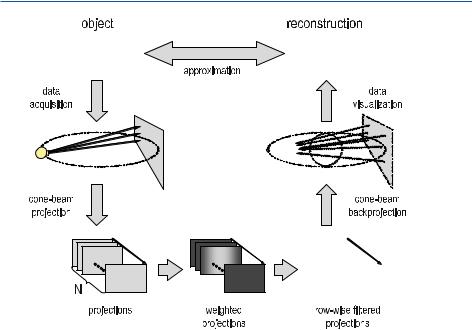
8.6 Approximate 3D Reconstructions in Cone-Beam Geometry

Fig. . . Schematic representation of the FDK method. It is an approximate X-ray conebeam reconstruction algorithm proposed by Feldkamp, Davis, and Kress

The FDK reconstruction method provides an exact backprojection instruction for the values measured in a plane including the circular X-ray source trajectory. Generally, the FDK reconstruction is of course an approximate method, since the Radon space is incomplete. It has already been pointed out in Sect. . . that the Tuy–Smith su ciency condition is not fulﬁlled for this trajectory.

For a point r = (x, y, z)T, which is located outside the (x, y) source plane to be reconstructed, all other projections related to a particular, arbitrarily selected projection fan-beam plane A are missing. Therefore, the objects located within this plane A cannot be exactly reconstructed. Some Radon data are always inaccessible due to the shadow zone illustrated in Fig. . for any point outside the (x, y) plane.

However, many studies have revealed that the deﬁciency of the FDK method due to the incomplete Radon data set of the planar X-ray source trajectory is only a minor deﬁciency, if the aperture angle of the cone beam is small. Figure . schematically shows a summary of the FDK method.

The exact three-dimensional X-ray cone-beam backprojection method proposed by Defrise and Clack, which was described in Sect. . . , was not formulated for a special source trajectory. Consequently, if ( . ) and ( . ) are compared, a certain relationship between the two di erent methods can clearly be seen. In both cases, the backprojection is deﬁned as an integral over the trajectory parameters, whereby a ﬁltered projection term h is used as integrand, weighted with the reciprocal, normalized squared distance (FCD U) of the projection of the distance

8 Three-Dimensional Fourier-Based Reconstruction Methods

between the point to be reconstructed and the X-ray source onto the central X-ray beam. In fact, it can be shown that the exact method proposed by Defrise and Clack is indeed reduced to an approximate FDK method, if a single circle is assumed to be the source trajectory S(λ) (Jacobson ).

8.6.3

FDK Cone-Beam Reconstruction for Cylindrical Detectors

Most of the detectors used today for medical applications are cylindrical detectors; therefore, the FDK approximation should be described for this geometry as well. Figure . shows the cone-beam geometry in the cylindrical detector arrangement with the fan angle ψ and the cone angle κ, which is deﬁned by

ε	.
κ = arctan FCD	.	( . )

With this deﬁnition, it is clear that the cone angle is constant along the individual rows (ε = const.) of the cylindrical detector. Figure . illustrates that ε = b only applies to the fan angle ψ = . In general, one ﬁnds the expression

b =	ε	( . )
	cos(ψ)
between the planar and the cylindrical detector arrangement.

Fig. . . Cone-beam illumination of a cylindrical detector. The X-ray source rotates on a radius FCD. A virtual detector is placed in the iso-center of the rotation of the sampling unit

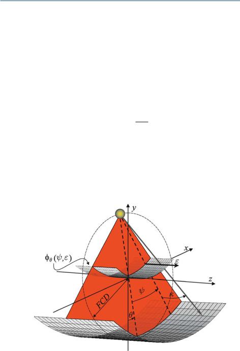
8.6 Approximate 3D Reconstructions in Cone-Beam Geometry

The individual lines of the detector are, of course, not located on a planar surface containing the X-ray source. Planar surfaces, which were used in the previous section, rather produce slightly curved intersections with the cylindrical detector. However, it is possible to re-interpolate the projection data so that they are located on a planar Cartesian grid.

The reconstruction method with cylinder geometry is split into three principal processing steps in Scheme . .

Finally, a few important properties of the FDK reconstruction method should be summarized.

•Exact reconstruction is ensured by the FDK method in the central radiation plane. This is, of course, the minimum requirement to be met by the method. ( . ) or ( . ) reduce to ( . ) or ( . ) respectively, for the corresponding

Scheme . FDK reconstruction with cylinder geometry

. Pre-weighting of the cylinder detector projection values

FCD

ϕθ (ψ, ε) = ϕθ

(ψ, ε)

cos (ψ)

( . )

FCD +ε

= ϕθ (ψ, ε)cos (κ)cos (ψ)

. Filtering of the projection signal. The ramp ﬁlter

g(ψ, ε) =

sin(ψ)

g(ψ, ε)

( . )

is a modiﬁed version of the ﬁlter for the parallel projection and is given in full

analogy to ( . ). Combined with the pre-weighting process described in the ﬁrst

step of this scheme, the high-pass ﬁltered signal for backprojection results from the

convolution in the angular domain

( . )

hθ (ψ, ε) = ϕθ (ψ, ε) g(ψ, ε) .

. Again, in analogy to the equations in

Sect. . . , the ﬁltered backprojection over

the full angle of π is given by

fFDK(x, y, z) =

∫

hθ

(ψ, ε)dθ ,

( . )

where

L = /

(FCD −x sin(θ) + y cos(θ)) + (x cos(θ) + y sin(θ))

( . )

is deﬁned as the distance between the X-ray source and the actual point to be reconstructed in the (x, y) plane.

8 Three-Dimensional Fourier-Based Reconstruction Methods

two-dimensional X-ray fan-beam reconstruction for the cone angle κ = (i.e., b = for the planar detector or ε = for the cylindrical detector).

•The larger the cone angle κ, the poorer the quality of the reconstructed image.

This is due to the fact that an increasing quantity of Radon data is located in the shadow zone (cf. Sect. . . ).

•The FDK method is exact for objects that are homogeneous in the z direction, i.e., for objects obeying f (x, y, z) = f (x, y). This result is achieved by pre-weighting with cos(κ) in ( . ) for the planar detector or ( . ) for the cylindrical detec-

tor. The longer path along which the X-ray beam is attenuated with a larger cone angle κ is weighted by the factor cos(κ) in such a way that the attenuation does not depend on the cone angle and corresponds to the attenuation in the central plane. The pre-weighted lines of the detector are identical for such objects, i.e., the method reduces itself to the fan-beam method in the plane.

Considering the planar detector, it should ﬁnally be pointed out that:

• The integral

pz = ∫ f (x, y, z)dz ( . )

is exactly preserved in spite of the approximate character of the FDK method. This is due to the fact that all surface integrals that are perpendicular to the central plane can be measured by a single planar, circular X-ray source trajectory, i.e., they are located within the measurable torus in the Radon space.

8.6.4

Variations of the FDK Cone-Beam Reconstruction

Weighting with the U− -factor in ( . ) is one of the problems related to the actual implementation of fast three-dimensional reconstructions. As very fast implementations for reconstruction algorithms in parallel-beam geometry are generally available, it seems to be useful to convert the cone-beam geometry into parallel-beam geometry by rebinning the beams in analogy to Sect. . . . As data are missing in the Radon space with the cyclic, planar source trajectory, this can be achieved successfully in the fan direction ψ, but not in the cone direction κ.

8.6.4.1

Rebinning with the Planar Detector

For the planar detector, the rebinned projection signal (without derivation, see Turbell [ ]) obeys

(

) =

(

) =

−

pγ

ξ, b

ϕγ−ψ

ψ, b

ϕγ−arcsin

ξ FCD

, b! .

( . )

FCD

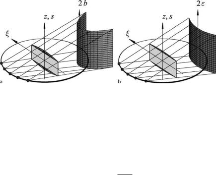
8.6 Approximate 3D Reconstructions in Cone-Beam Geometry

Fig. . . Geometry of the projections after the X-ray cone beams have been rebinned, for a the planar and b the cylindrical detector. In the iso-center of the rotation the virtual planar detector is illustrated (courtesy of Turbell [ ])

The coordinate of the detector line b remains unchanged here. If one considers this situation from the direction of the z coordinate, parallel-beam geometry has been achieved after completion of the rebinning process. The beams of a particular detector line b match a vertical planar detector (ξ, s) in the iso-center of the rotation along the curves

s(b, ξ) = b −	ξ	.	( . )
	FCD

Additionally, Fig. . a illustrates what a detector (which is also a virtual detector) would look like, if all beams of a particular detector line b had the same z value.

8.6.4.2

Rebinning with the Cylindrical Detector

For the cylindrical detector the rebinned projection signal – in analogy to ( . ) – obeys

pγ (ξ, ε) = ϕγ−ψ (ψ, ε) = ϕγ−arcsin	ξ	arcsin	ξ	, ε .	( . )
			FCD
	FCD

The coordinate of the detector line ε remains unchanged here. If one again considers this situation from the direction of the z coordinate, parallel-beam geometry has been achieved after completion of the rebinning process. The beams of a particular

detector line ε match a virtual planar detector

(

ξ, s

)

in the iso-center of the rotation

along the curves

(

) =

εl

−

FCD

ε, ξ

( . )

The intersection curves on the virtual, cylindrical detector are obviously not as curved as they are for the planar detector, as described in ( . ).

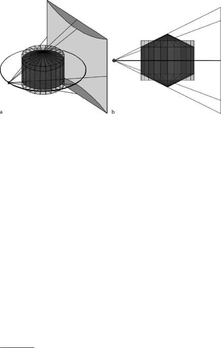
8 Three-Dimensional Fourier-Based Reconstruction Methods

Fig. . a,b. Once the data have been rebinned, the geometry of the illuminated volume is similar to a tent with a rectangular base area (courtesy of Turbell [ ])

8.6.4.3

Tent-FDK Method

Although one is able to accelerate the backprojection process by rebinning the data as described above, the artifacts are still the same (Turbell ). However, this changes if one takes into account the approach of Grass et al. ( ). They proposed to re-interpolate the data pγ (ξ, b) from ( . ) or the data pγ (ξ, ε) from ( . ), on the virtual (ξ, s) detector in the iso-center of the rotation in such a way that they lie on horizontal lines.

This method can only be applied reliably, i.e., a ramp ﬁlter can only be applied along horizontal lines, if the data along these lines on the detector are complete. Figure . a shows that the data in the shaded area may therefore not be used for the so-called T-FDK method . In Fig. . b, it can be seen that the cross-sectional area produced with the T-FDK method in the three-dimensional space is shaped like a tent with a rectangular base area. In practical applications, it is thus possible to reduce the radiation dose by suitable collimation of the required data. The T-FDK method is able to improve the quality of the reconstructed image.

8.6.4.4

Sequential FDK Method

Köhler et al. ( ) suggested sampling the patient projection data not on a helical path but in discrete distances Z on circular paths. If the real detector is high enough so that a virtual detector in the iso-center of the rotation has just the

T-FDK is the abbreviation of Tent-FDK, because the data form a tent after completion of the rebinning process.

8.6 Approximate 3D Reconstructions in Cone-Beam Geometry

Fig. . . The beam geometry of the sequential FDK method (S-FDK) is a straightforward extension of the FDK method in the axial direction (courtesy of Turbell [ ])

height Z, then all voxels receive exactly one backprojection contribution from each projection angle. Figure . is displaying this arrangement.

The voxels inside the double cone shown in Fig. . b receive their backprojection contribution from the source trajectory with the smallest distance to this voxel. All other points to be reconstructed receive contributions either from this trajectory or from the following circular trajectory. A point is illuminated from the consecutive circular trajectory at a projection angle θ+π only, if it is not illuminated at a projection angle θ from the nearest neighboring circular trajectory. According to this sequential FDK (S-FDK) principle, a complete set of measured projection values is made available for all points to be reconstructed.

8.6.4.5

FDK-SLANT Method

Within the original FDK method, a horizontal line on the (planar) detector at a particular projection angle θ is considered for a point to be reconstructed. This line is related to a projection plane A, which also contains the X-ray source and the point itself. The projection values on the detector line can be pre-weighted, ﬁltered, and then backprojected in the direction of the X-ray source in the plane, independent of all other projection angles and all other angulations, κ. If one switches over to another projection angle θ , one has to leave this plane and search for a new plane, which starts from the X-ray source and then runs through the point to be reconstructed at another angulation angle κ .

Turbell ( ) proposed to vary the FDK method in such a way that the plane is held when the projection angle changes. Figure . a shows a fan consisting of

8 Three-Dimensional Fourier-Based Reconstruction Methods

Fig. . a,b. The beams of the FDK-SLANT method have a geometrical pattern that is similar to the pages of a book. The intersection line between a book page and the detector plane is non-horizontal. This line on the (ξ,s) detector corresponds to the ﬁltering direction (courtesy of Turbell [ ])

held planes with horizontal intersection lines on the planar detector and touching the X-ray source trajectory at the projection angle θi at the point

Si = (−FCD sin(θi ), FCD cos(θi ), ) .

( . )

This geometrical situation is similar to a half-opened book, the pages of which are stitched together at the point Si in ( . ). Turbell then uses a number N of such books with the anchor points Si , with i = , . . . , N being uniformly distributed on the cyclic source trajectory. The ﬁrst ﬁve anchor points are shown in Fig. . b.

The ﬁltering direction of a ﬁltered backprojection at the projection angle θ is given by the intersection line of the detector plane and the book page with the anchor point Si . Figure . b clearly illustrates that the intersection lines on the virtual detector are slanted straight lines. The key idea of this method is that the backprojection is to remain as far as possible an interaction between the points within a single plane.

8.7

Helical Cone-Beam Reconstruction Methods

In the previous sections of this chapter, object reconstruction with cone-beam geometry based on initially arbitrary source trajectories (exact methods proposed by Grangeat, Sect. . . , and Defrise and Clack, Sect. . . ) and then special circular, cyclic X-ray source trajectories (approximate methods proposed by Feldkamp, Davis, and Kress and their extensions, Sect. . ) have been discussed. The derivative-free reconstruction method proposed by Feldkamp et al. ( ) has been

				8.7 Helical Cone-Beam Reconstruction Methods
frequently used in technical applications. However, it is an approximate method, the
use of which in medical applications is not unproblematic due to the required image
quality. As long as the cone angle aperture of the X-ray beam is small, this method
yields acceptable results. However, today, the development of new detector genera-
tions focuses on even larger ﬂat-panel detectors; thus, the reconstruction algorithms
must be adapted accordingly. Also, inherently three-dimensional methods must be
implemented because the three-dimensional adaptations of the two-dimensional
approaches reach their limits.
	In			Sect. . . it has been explained that a single circular, cyclic source trajec-
tory		cannot completely ﬁll the Radon space. As Kalender et al. ( ) has success-

fully demonstrated with the spiral method for the one-dimensional detector array
(cf.			Sect. . ), here it can be shown that the methods developed for cone-beam

geometry can be adapted to spiral or helical trajectories
				S(λ) = (−FCD sin(λ), FCD cos(λ), hλ)	( . )

of the X-ray source. In Fig. . it has already been illustrated that the helix represents an X-ray source orbit, which, in principle, may completely ﬁll the Radon space. In this case, λ ; Λ R is again the parameterization of the trajectory. The parameter h denotes the rise of the helix. The parameter pitch introduced in Sect. . , explaining the simple spiral CT method, has no direct meaning in an X-ray cone. However, the pitch parameter can be adapted to the new situation. This can be done for instance by deﬁning P = πh, meaning the table feed in z direction per full rotation of the sampling unit on the gantry (Proksa et al. ). In this way, the patient

Fig. . . Tam–Danielsson window B on the ﬂat-panel detector array ϕλ (a, b), which is exceptionally located outside the source trajectory area here. The data window B on the detector used for the reconstruction process is deﬁned by two successive arcs of the spiral. It is called a PI window

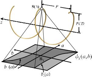
8 Three-Dimensional Fourier-Based Reconstruction Methods
table feed in the axial direction can be expressed by
	P
z(λ) = λ		+ z .	( . )
	π

Figure . illustrates the geometrical situation. The detector is exceptionally not placed in the iso-center of the helical rotation, although the mathematics of the object reconstruction would be more concise if a virtual detector were considered in the iso-center.

The data measured by a rectangular ﬂat-panel detector must be windowed to prevent projection values being overrepresented in the reconstruction algorithm. For this purpose, one only considers the detector ﬁeld in the area B. T he so-called Tam–Danielsson window (Tam ; Turbell ) is deﬁned by restricting the X-ray beams to the area between two successive spiral arcs opposite the source position S(λ). On the planar (a, b) detector with the projection values ϕλ (a, b), a projection yields the restriction of the data to be used between the curves

( ) =

arctan

a FCD

+π

( . )

FCD

)

(

= h +

arctan (a FCD) +

FCD

and

( ) =

−π

arctan

a FCD

( . )

b−

FCD

)

(

= h + FCD arctan (a FCD) − .

Due to this restriction, this method is classiﬁed as a so-called PI method.

The object may now be reconstructed according to the approach proposed by Pierre Grangeat, which has been described in Sect. . . . For this purpose, the derivative of the three-dimensional Radon transform, i.e., the di erentiation of the integration over the Radon surfaces through the object, has to be computed. Figure . shows the orientation of an arbitrary Radon surface through the object. As the aperture of the X-ray cone is limited, the Radon surface must be assembled from several segments.

The points of intersection of the helical X-ray source orbit with the Radon surface in consideration (cf. Fig. . a) are the nodes of a triangulation of the Radon surface. In Fig. . b, visualization along the surface normal of the Radon surface onto the resulting triangulation is given. The Tam–Danielsson window restricts the measured values in such a way that each triangle is illuminated exactly once. Thus,

8.7 Helical Cone-Beam Reconstruction Methods

Fig. . . a The intersection points of the helix are basis points by means of which any Radon surface may be triangulated. b If one looks perpendicularly onto the Radon surface, one sees the segments of the Radon surface, which is thus completely illuminated, but not in an overlapping manner

if the source has reached the position S(λ ), then the data made available are restricted by the points S(λ ) and S(λ ) in accordance with ( . ) and ( . ), so that the corresponding triangle is exclusively illuminated by the X-ray source at position S(λ ). If one assembles all these segments, an angulated ellipse can be found within the helix (cf. Fig. . a).

The key idea of the exact reconstruction for incomplete projections is the combination of the individual contributions of the segments shown in Fig. . . The intermediate result of Grangeat was

∂				∂		Tμγ,ϑ (σ, τ(ξ))U dσ ,
	pγ,ϑ (ξ) =		−∫		Xwc		( . )
∂ξ		cos (κ)		∂τ

i.e., replacing the derivative in the radial direction of the Radon transform with the weighted radial detector derivative and line integration.

The surface can be decomposed into triangular segments

∂

Tμγ,ϑ (σ, τ(ξ), λi )U dσ ,

pγ,ϑ (ξ, λi )

σ∫

Xwc

( . )

∂ξ

cos (κ)

∂τ

whereby the sum over all N triangular elements

∂

( ) =

∂

(

)

pγ,ϑ

ξ, λi

( . )

∂ξ

i =

∂ξ

only yields the desired derivative of the Radon transform.

8 Three-Dimensional Fourier-Based Reconstruction Methods

Kudo et al. ( ) have shown that the single addition in ( . ) unfortunately does not provide an exact reconstruction result. They proposed a correction term

∂	pγ,ϑ (ξ, λi ) =		σ	∂		Tμγ,ϑ (σ, τ(ξ)), λi U dσ + . . .
			∫		Xwc
∂ξ		cos (κ)		∂τ

ċċ ċ − tan(κ) σ Xwc Tμγ,ϑ (σ , τ(ξ))U − σ Xwc Tμγ,ϑ (σ , τ(ξ)), λi U

FCD

( . )

considering the actual borders of the integration intervals. Turbell ( ) interprets this correction term as a compensation of a minor change in the triangular surface, which arises when the Radon surface moves along the surface normal, while the derivation process is carried out. On the basis of this piece of Radon data, the ﬁltered backprojection may, for instance, now be implemented according to the approach proposed by Defrise and Clack ( ).

Proksa et al. ( ) have shown that this PI method can of course be extended to a n-PI method, if larger ﬂat-panel detector areas are used. If one deﬁnes the detector window more generally as

( ) =

−

arctan

a FCD

( . )

bn a

FCD

)

(

= h +

nπ

− arctan (a FCD)

FCD

where

Bn = (a, b) − bn (−a) b bn (a) ,

( . )

the data used cover a multiple of the helix pitch. This extension is called the n-PI window .

The ellipse resulting from a section of the Radon surface under consideration with the helix contains an odd number no of piercing points, S(λi ), of the source trajectory with the Radon surface. For the n-PI detector Proksa et al. ( ) found that all Radon surfaces with no piercing points and no < n have an no-fold illumination or over-representation. If no : n, the Radon surfaces have an n-fold over-representation. The corresponding over-representation is compensated for by means of a function M, which has already been mentioned in Sect. . . .

All positive integer odd numbers are in principle acceptable in this context. But in practice, only n = , , , and are used.

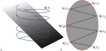
8.7 Helical Cone-Beam Reconstruction Methods

In the case here, the M function reads
						for no	(	λ, nξ	) <	n ,
	(		) = /		)		(		) <
Mn		λ, nξ	- no	λ, nξ							( . )
			.
			.
			0			otherwise
			.			otherwise

so that one may ﬁnally formulate the reconstruction shown in Scheme . .

Today, a multitude of algorithms or implementation strategies are available for three-dimensional helix-based X-ray cone-beam geometries.

Finally, the rebinning strategy, which has already been formulated for a tilted gantry (Kachelrieß et al. , ), should be addressed. Compared with the n-PI methods, the essential di erence is due to the possibility of replacing the computationally expensive, three-dimensional backprojection step with a two-dimensional backprojection step on appropriately deﬁned planes. The appropriate slice is deﬁned such that its inclination matches the helical X-ray source trajectory locally.

Scheme . Exact cone-beam helical reconstruction for n-PI detector geometry

. Determination of the number of intersection points no with the helix for all Radon surfaces.

. Computation of the positions S(λi ) for all intersection points from step .

. Determination of the integration intervals [σ , σ ]belonging to the individual positions.

. Computation of the derivative of the individual partial Radon surfaces

∂

&μγ,ϑ (σ, τ(ξ)), λi ' dσ + . . .

pγ,ϑ (ξ, λi ) =

σ∫

∂ξ

cos

(

)

∂τ

. . .

−

tan(κ)

σ Xwc

μγ,ϑ

(

, τ ξ

, λi

' +

. . .

( . )

FCD "

( ))

. . . −

σ Xwc

&μγ,ϑ (σ , τ(ξ)), λi '# .

. Computation of the compensation function

Mn(λ, nξ ) =

( . )

min no(λ, nξ ), n

. Summation of the individual Radon segments

∂

(

) =

∂

(

)

pγ,ϑ

ξ, λi

( . )

∂ξ

= ∂ξ

. Computation of the object with the Radon inversion formula

(

x, y, z

∫∫S

∂ pγ,ϑ (ξ)

dS .

( . )

) = − π

∂ξ

8 Three-Dimensional Fourier-Based Reconstruction Methods

As illustrated in Fig. . the two-dimensional reconstruction plane nutates about the patient z-axis like a gyroscope with an inclination angle, α. T he nature of the di erent reconstruction artifacts is described by Köhler et al. ( ).

As a last remark regarding helix-based cone-beam geometry, it should be mentioned that Katsevich ( ) proposed an exact backprojection method that also works for long objects in such a way that one does not have to include data acquired in areas far away from each other.

Fig. . . Nutation of the two-dimensional reconstruction plane around the axial direction. The surface normal is tilted by the angle α with respect to the axial direction

Fig. . . Performance of modern cone-beam CT scanners with ﬂat-panel detectors. a and b show the three-dimensional visualization of a human jaw and a corresponding section through a row of teeth. c shows the smallest human bones, i.e., the hammer, anvil, and stirrup in the middle ear. The pictures have an isotropic spatial resolution of μm (courtesy of General Electric Medical Systems: Pfoh [ ])

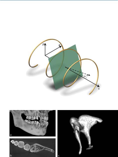
8.7 Helical Cone-Beam Reconstruction Methods

Figure . demonstrates the performance of a cone-beam CT prototype scanner. The scanner is equipped with a ﬂat-panel detector measuring cm cm with. . detector elements (cf. Sect. . . ). Figure . a shows the volume CT image of a human jaw. Figure . b shows the corresponding section through a row of teeth, revealing extremely small details with a resolution of μm. Even the smallest bones in the human body, i.e., the hammer, anvil, and stirrup in the middle ear, can be excellently imaged with an isotropic spatial resolution of μm. Figure . c shows a volume CT image of the three bones (Pfoh ).

<<< < Предыдущая 1 2 34 / 74 5 6 7 > Следующая >>>

Соседние файлы в предмете [НЕСОРТИРОВАННОЕ]

#
25.04.201979.36 Кб1Boiler_and_reactor_building_Unit4.doc
#
29.05.201519.47 Кб32Brass.docx
#
29.05.201526.89 Кб22Buddizm.docx
#
29.05.20151.2 Mб34Bukhgaltersky_uchet_UP_2012.doc
#
29.05.20156.06 Mб3107BusinessEnglish_Nikolaenko.pdf
#
29.05.201515.29 Mб42Buzug_Computed_tomography_From_photon_stat.pdf
#
29.05.2015403.08 Кб23BZhD_otvety-1.pdf
#
17.09.2019822.27 Кб11bzhd_otvety.doc
#
23.11.2019302.59 Кб6b_12101809_t_k_r_fizika.doc
#
25.08.20191.49 Mб69C2.doc
#
29.05.20151.42 Mб27CFZ_TREBOVANIYa.doc