Добавил:

Upload Опубликованный материал нарушает ваши авторские права? Сообщите нам.

Вуз:

Томский Политехнический Университет

Предмет:

[НЕСОРТИРОВАННОЕ]

Файл:

Buzug_Computed_tomography_From_photon_stat.pdf

Скачиваний:

Добавлен:

29.05.2015

Размер:

15.29 Mб

Скачать

☆

<<< < Предыдущая 1 23 / 73 4 5 6 7 > Следующая >>>

6Algebraic and Statistical Reconstruction Methods

Contents

6.1 Introduction . . . . . . . . . . . . . . . . . . . . . . . . . . . . . . . . . . . . . . . . . . . . . . . . . . . . . . . 201

6.2 Solution with Singular Value Decomposition . . . . . . . . . . . . . . . . . . . . . . . . . . . . . . . 207

6.3 Iterative Reconstruction with ART . . . . . . . . . . . . . . . . . . . . . . . . . . . . . . . . . . . . . . . 211

6.4 Pixel Basis Functions and Calculation of the System Matrix . . . . . . . . . . . . . . . . . . . . . 218

6.5 Maximum Likelihood Method . . . . . . . . . . . . . . . . . . . . . . . . . . . . . . . . . . . . . . . . . . 223

6.1 Introduction

Currently, the ﬁltered backprojection (FBP) method, which has been discussed inSect. . , is the reconstruction algorithm of choice because it is very fast, especially on dedicated hardware. However, one disadvantage of FBP is that it essentially weights all X-rays equally. Since X-ray tubes produce a polychromatic spectrum, beam-hardening image artifacts arise in the reconstruction. Artifacts of this type are particularly dominant if metal objects are inside the patient, because FBP interprets the corresponding projection data as inconsistent. Here, algebraic and statistical reconstruction methods will serve as alternatives because artiﬁcial or inherent beam weighting reduces the inﬂuence of rays running through metal objects.

Algebraic and statistical methods for computed tomography (CT) image reconstruction are widely disregarded in clinical routine due to the substantial amount of inherent computational e ort. On the other hand, the continuously growing computational power of today’s standard computers has led to a rediscovery of these methods.

At the advent of CT, the ﬁrst image reconstructions were carried out using algebraic reconstruction techniques (ART). As mentioned above, in today’s clinical routine FBP is the working horse of CT image reconstruction due to the computational expense of ART . However, ART is more instructive since it represents the reconstruction problem as a linear system of equations.

Today, special iterative statistical techniques are widely used in nuclear diagnostic imaging in order to overcome the problems in the signal-to-noise ratio caused by poor photon statistics.

6 Algebraic and Statistical Reconstruction Methods

Generally, these methods are much easier to understand than the Fourier-based strategies discussed so far. Thereby, one takes the discrete nature of the practical realization of CT into account from the very beginning. Discretization of the projection, pγ (ξ), is technically dictated by the design of the detector array based on a set of discrete detector elements. The discretization of the tomographic image, i.e., the size and number, N, of pixels inside the ﬁeld of view, has to be determined before image reconstruction can take place. Figure . shows the situation of spatially discrete attenuation values schematically. The tomographic image that has to be reconstructed, however, consists of a discrete array of unknown variables, f j, with j = , . . . , N , i.e., the unknown attenuation coe cients. The set of projections through the object can easily be modeled by a linear system of equations. Figure . motivates this set-up of a linear system of equations. Passing through tissue, the intensity of the X-ray beam is weakened according to the attenuation coe cients, f j = μj . If the image is small, the solution of the corresponding low dimensional linear system of equations can be obtained, for example, by Gaussian elimination (cf. Press et al. [ ]).

For each ray through the object, one obtains the already known projection sum deﬁned in Sect. . and, furthermore, the following system of equations for the situation of the -pixel image in Fig. . a.

f	f	p ,	( . )
f	+ f	= p ,	( . )
f	+ f	= p ,	( . )
	+	=	( . )
f + f		= p ,	( . )

Fig. . . The principle of algebraic reconstruction is very simple. The set of projections results in a linear system of equations. In the left image all four unknown attenuation values can be determined exactly using four projections from three projection angles. If the grid that is to be reconstructed is ﬁner, more projections have to be measured

6.1 Introduction

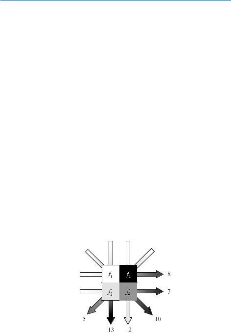
Four equations are obtained with four unknown quantities that can be solved exactly, as long as the physical measuring procedure is not a icted with noise and no linear dependencies occur – that is as long as the rank is in the example above . Now the image shall be reﬁned spatially as demonstrated with the -pixel image in Fig. . b. It is immediately clear that the number of required independent X-ray projections grows quadratically with the linear reﬁnement of the image. In the given example, one obtains a solvable problem consisting of nine equations and nine unknown attenuation values. Looking at the diagonal projections, a di erence is apparent compared with the horizontal or the vertical projection direction: The path length through each element of the object is obviously di erent. This circumstance must be taken into account in the set-up of the system of equations.

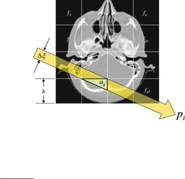
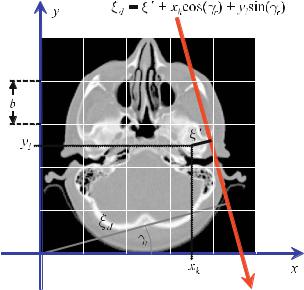
In contrast to the methods introduced in the previous chapter, in which the object is sampled with a δ-line, when using algebraic methods, one proceeds with the physically correct assumption that the X-ray beam has a certain width. When passing through tissue, one now has to take into account how much of the pixel that is to be reconstructed is passed through by the beam. For this purpose, one introduces weights that reﬂect the relation between the area that is illuminated by the beam and the entire area of the pixel. Figure . shows this ratio schematically. A beam of

Fig. . . The X-ray beam of width ξ does not traverse all pixels of size b equally when passing through the tissue. The area of the pixel section that has actually been passed through and that is to be reconstructed must be included in the system of equations as a weighting

This is true if a diagonal projection through the object is involved. Two horizontal and two vertical projections alone would lead to an under-determined system of equations having a rank of .

6 Algebraic and Statistical Reconstruction Methods

width, ξ, passes through the tissue – again illustrated by cranial tomography. T he pixel size is given by b . T he weightai j is thus determined by the relation

	ai j	=		illuminated area of pixel j by ray i					( . )
	ai j	=			total area of pixel j				( . )
and lies in the interval			ai j .
From the	generalizations of ( . ) to ( . ), one obtains the following system of
From the
equations:
					N		=
						ai j f j	=	pi ,	( . )
						ai j f j		pi ,	( . )

j =

in which the weights, ai j, are taken into account. N is the number of the pixels, n , that are to be reconstructed, and i = , . . . , M is the index of the projection, with M = Np D being the total number of projections of all detector elements, D, of the detector array in all projection directions, Np. In an expanded form, one may write ( . ) as

a f + a f + ċċ ċ + a N a f + a f + ċ ċċ + a N

aM f + aM f + ċ ċċ + aMN

fN		p
fN	= p
fN V=		pM .	( . )
	=

Within nuclear diagnostic imaging, as in PET and SPECT , in which the representation of the photon paths as a set of linear equations is used in a statistical approach, the weightings are to be interpreted as probabilities that gamma quanta from the area element j are detected in projection i. This shows the strength of the algebraic and statistical techniques. Linear physical processes can be built into the imaging model via appropriate weightings of the projection equations. In this way, the imaging quality can be improved because the mathematical model that the reconstruction is based on can be tailored to match the real physical situation.

Writing all projections as column vector

p = (p , . . . , pM )T ,

( . )

and writing the attenuation values that are to be reconstructed as a column vector as well (they were presented as an image matrix in the previous sections)

	f = (f , . . . , fN )T ,	( . )

To be precise, this deﬁnition is only exact in the case of emission CT.
PET = Positron Emission Tomography.
SPECT = Single Photon Emission Computed Tomography.
Physically, the gamma quanta emerge from a volume element.

						6.1	Introduction
the weightings are thus presented as an M N matrix
	a	a . . .		a N	!
A	a	ċ		a N	!	,	( . )
	= aM	ċ	ċ	aMN	"
	V		ċ	V	"
such that the system of equations becomes					#
such that the system of equations becomes
	p = Af ,						( . )

where A can be understood as design matrix (Press et al. ). In CT, this matrix is also referred to as the system matrix (Toft ). Through a direct comparison with ( . ) the following duality between the presentation as matrix and the Radon transform can be identiﬁed:

p	= A		(	f	)	( . )
(	) = R	f	(	xW, y	)
pγWξ	W	f		xW, y

Therefore, vector p contains all values of the Radon space, which means it contains all values of the sinogram, and f is the vector that contains all gray values of the image grid, i.e., the attenuation coe cients. The mathematical di culties in this view on the reconstruction problem can be summarized by the following points:

•The system of equations ( . ) can only be solved exactly under idealized

physical conditions. In the present case, however, one has to deal with real data, i.e., data a icted with noise. Therefore, even in the case N = M, only

an approximate solution can be found for f. Furthermore, for high-quality CT scanners it is true that M N, which means that the number of projections is higher than the number of pixels that are to be reconstructed. Mathematically, this situation leads to an over-determined system of equations.

•Typically, the system matrix, A, is almost singular, which means that it contains very small singular values such that the reconstruction problem is an ill-conditioned problem.

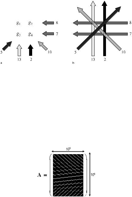
•A does not have a simple structure and so no fast inversion has been found so far. On the other hand, A is a sparse matrix as only N pixels contribute to an entry in the Radon space (cf. Fig. . ).

•A is usually very large, so direct inversions are extremely timeand memory-intensive (cf. Fig. . ).

6 Algebraic and Statistical Reconstruction Methods

However, there are interesting advantages of the algebraic approach as well:

•Irregular geometries of scanners or missing data in the sinogram lead to severe di culties in the direct reconstruction methods. In the matrix formalism, however, these geometric conditions can be considered and taken into account adequately.

•Finite detector widths and di erent detector sensitivities can be taken into account. Therewith, better modeling of the real physical measurement process can be obtained.

•Beams running through objects that potentially produce inconsistencies in the Radon space can be weighted appropriately.

The solution of ( . ) can generally be found by minimization of the following function

χ = Af − p .

( . )

There is always a solution for this optimization problem. The solution is called the least squares minimum norm or pseudo solution. One thereby searches for a matrix called the pseudo inverse A+ of A, also called the Moore–Penrose inverse (Natterer), with the following properties:

AA+A = A

A+AA+ = A+

(AA+)T = AA+ ( . ) (A+A)T = A+A

In a certain sense, A+ represents the inverse matrix to the square matrix A such that
Xf = A+p .	( . )

As the pseudoX solution ( . ) is a compromise in the least squares sense, it is denoted by f.

With respect to the duality between the matrix presentation and the Radon transform equation,

g = ATp

( . )

presents the adjoint Radon transform of sinogram values to the image space. ( . ) represents the unﬁltered backprojection that is analogous to ( . ).

( . ) can be brought into standard form by multiplying with AT from the left, thus

This leads to the solution	ATp = ATAf .	( . )
	f = (ATA)− ATp .	( . )

6.2 Solution with Singular Value Decomposition

Interestingly, ( . ) can be discussed in the language of the Fourier-based reconstruction methods. In the sense of the adjoint Radon transform ( . ) mentioned above, here matrix AT represents the backprojection operator and, consequently, the operator (ATA)− represents the necessary ﬁltering. As discussed in Sect. . , it is indeed sensible to perform a simple backprojection prior to the ﬁltering. Obviously, this leads to the layergram method so that ( . ) can be seen in duality to ( . ). However, it is also possible to represent the ﬁltered backprojection discussed in Sect. . as a matrix equation.

Starting with ( . ), some rearrangements lead to the following result:

ATA

− ATp

AAT

− p

= (ATA)− AT

AAT

)(

= (

)

(

)

( . )

ATA −

ATA AT AAT − p

AT AAT − p .

(

)

= (

(

) (

)

Here, the term

AAT − plays the role of the high-pass ﬁlter q

from ( . ). So the

pseudo inverse

(A+ is )given by

A+ = AT(AAT)− = (ATA)− AT

( . )

and is determined practically by singular value decomposition.

6.2

Solution with Singular Value Decomposition

Using singular value decomposition (SVD) to solve ( . ) needs the CT system matrix to represent the design matrix, A, in the following system of equations:

( . )

p ! .

Within SVD any M

N matrix A with M

N, can be decomposed into

where U is an M N

diag

VT ,

( . )

A UΣV

orthogonal matrix and V is an N N orthogonal matrix in

columns being orthonormal. Σ is a diagonal N

N matrix whose

the sense of their

entries are the singular values σj. One obtains the pseudo inverse of A through

A+ = V diag σj

UT .

( . )

6 Algebraic and Statistical Reconstruction Methods

In that way, the solution of ( . ) can be found by								!	p! .
f!	V	!	σ	ċ		!	UT	!	p! .	( . )
" =		"	ċ ċ ċ			"		"	"
#		#		ċ		#		#	"
X					σN

To illustrate the principle, an X-ray illumination from four directions of an object is given schematically in Fig. . . The image will be reconstructed as a pixel image.

The system of equations belonging to Fig. . is the concretization of ( . ), thus

"	f		!		"
"	f		!		"
!		f	"		!
"	f		"	=	"
"			"		"
"		f	#		" .	( . )
"			#		"
#					#

Here, the nearest neighbors method was used to calculate the weights, ai j, represented in the system matrix. Di erent methods for the determination of weights that are more appropriate to the physical situation will be explained in the next section. The system of equations ( . ) is over-determined, which means that there are more equations (projections, pi ) than unknown quantities (pixel values, f j). Obviously, some of the rows in this system are linearly dependent. The number of linearly independent equations can be expressed by the number of non-zero singular values. This number gives the rank of the matrix, A.

With the singular value decomposition described above, one obtains the pseudo inverse that solves the system of equations. Matrix A hereafter contains four ﬁnite

Fig. . . Example of an object that is irradiated from four directions. Six projection values are acquired. T he image will be reconstructed as a pixel image. A linear black to white lookup table simulates weak to strong attenuation

6.2 Solution with Singular Value Decomposition

singular values and is thus of the rank . The singular values are σ

. and

. . With the decomposition presented in ( . ),

one obtains the

pseudo inverse

−

A+

( . )

−

so that ( . )−

−

	!			!
				!
				""
f		=	A+	"	( . )
X=	"	=		"
	"			"
	#			"
				#

is the solution in the least squares sense. A comparison with Fig. . indicates that ( . ) does indeed provide the correct solution.

Unfortunately, in practice, the solution of the system of equations ( . ) cannot easily be obtained, because typically, the problem is ill-conditioned, i.e., very small singular values, σ , might occur. In consequence, even small measurement errors in the projections, pj, may induce large ﬂuctuations in the reconstructed image, Xf. In these cases, the solution has to be stabilized with a technique called regularization. Press et al. ( ) suggested weighting the spectrum of the singular values appropriately. In the easiest case, σj is replaced by a zero if σj exceeds a certain threshold.

Finally, the example of ( . ) will be considered again from the perspective of the adjoint reconstruction problem ( . ). To do so, one has to transpose the system matrix, A, and write

g !
	g	"	=
g		"	=
	g	"
		#

	!
	!
"	"	=	"
"	"	=	"	( . )
!	"		! .	( . )
"	"		"
	"		#
#	"		#
	#

As argued above, ( . ) presents the unﬁltered backprojection. Figure . illustrates the method schematically, using the sample data from Fig. . .

So far it has been shown that, in principle, the direct algebraic method leads to an exact image reconstruction using SVD. If the number of projections, M, and the number of pixels, N, to be reconstructed are small, the system of equations ( . ) can actually be solved directly. In the example ( . ) it has been chosen that M = and N = . However, it must be clear that in modern CT scanners the real physical situation is given by a very large system of equations. Even computers of the latest generation are not prepared to solve the problem with such a method of brute force.

	6 Algebraic and Statistical Reconstruction Methods

Fig. . a,b. Schematic presentation of the adjoint problem g = ATp to equation p = Af. T he adjoint reconstruction problem presents the unﬁltered backprojection

A modern CT system typically has about . detectors in a single detector slice and acquires just as many projections in a -rotation such that M is in the order of . For an image matrix of pixels that is to be reconstructed, N is to the order of . In Fig. . , it is illustrated that the system of equations ( . ) to be solved consists of unknown quantities and equations. That is why all practicable algorithms for the solution of the linear system of equations work with iterative concepts that do not need a direct inversion of matrix A.

It should be noted that if the linear system of equations ( . ) could be represented in diagonal form, the solution could be directly determined. Indeed, the Fourier-based methods can be interpreted in such a way that the Fourier transform reduces the reconstruction problem to a diagonalized system of equations. That is why the Fourier methods are very e cient (Epstein ).

Fig. . . The system matrix, A, is a huge but sparse matrix. The structure of entries of A is given in gray dots. Since modern CT scanners produce an image matrix of at least pixels, N is in the order of . Usually, a single-slice detector array consists of detector elements and data are acquired from projection angles. This leads to a matrix size ofelements

6.3 Iterative Reconstruction with ART

6.3

Iterative Reconstruction with ART

ART stands for algebraic reconstruction technique. In fact, Hounsﬁeld used this method for the ﬁrst CT image reconstructions. While doing so, as mentioned before, he was not acquainted with Radon’s publication in . However, later it became clear that iterative ART is a reinvention of Kaczmarz’s method published in(Kaczmarz ).

The methods, which use iterative strategies to solve ( . ), usually start with the

notion that the realization of an image, f

f , . . . , fN

T, presents a point in an

N-dimensional solution space. Starting with an initial image, f( )

, a sequence of

images,

), f(

), . . .

= (

)

, is calculated iteratively that converges to the desired tomo-

graphic reconstruction.

In the ﬁrst step, a forward projection,

p(n) = Af(n),

( . )

of the nth image approximation f(n) is determined. The projection, p(n), determined in the nth forward projection can then be compared with the actual measured projection, p. The comparison between the determined and the measured projection yields correction terms that are applied to the nth image approximation, f(n), resulting in the (n + )th image approximation. This process is iteratively repeated such that with another forward projection, the projection p(n+ ) is determined.

Usually, iterative methods are structured into three categories (Schramm ):

•Methods with correction of all object pixels at the same time: In this case all of the corrections are determined in one step using all information contained in the projection data set. By doing so all object pixels are corrected at the same time. Iterative Least Squares techniques (ILST) belong to this category, as well as the maximum likelihood methods, which will be discussed below.

•Methods with pixel-wise correction: In this category all pixels of the nth iteration are corrected one after the other. For the determination of the correction term only the projection elements to which the relevant pixel made a contribution in the forward projection are consulted.

•Methods with beam-wise correction: Methods like ART operate by using the information of only one beam sum. Then the object pixels that made a contribution to the appropriate projection pixel are corrected. Afterward the determination of the next beam sum follows. ART is therefore sometimes called the ray-by-ray reconstruction method.

An example ﬁrst published by Kak and Slaney ( ) and Rosenfeld and Kak ( ) is repeated here to illustrate the idea of the correction using the strategy of

6 Algebraic and Statistical Reconstruction Methods

beam-wise methods. The N-dimensional solution space in which the realization

of an image, f

f , . . . , fN

T, is optimized, is divided into M hyperplanes given

of equations ( . ). If there is a unique solution of ( . ) or ( . ), the

by the system

= (

)

= (

intersection of all hyperplanes will result in a single point, namely f

, . . . , fN ) ,

that represents the solution.

For illustration, the dimension of the problem is reduced to N

, which

projections are

means the desired image consists of two pixels and two measured=

available. The corresponding system of equations is

a f

( . )

+a f

= p

In Fig. . the iterative solution scheme can be understood graphically.

As a starting point, one needs an initial image, f( ), as a base for which the iteration shall be started. This image could result from a rudimentary backprojection, for example. However, an image that is equivalent to the zero vector, f( ) = ( , , . . . , )T, serves the purpose equally. This vector is projected perpendicularly onto the ﬁrst straight line that represents the ﬁrst X-ray beam with the projection result, p , in order to obtain a new and improved image, f( ). This image is then projected perpendicularly onto the second straight line. Therewith, one obtains an image that is improved with respect to f( ) because f( ) lies closer to the intersection point of the straight lines than its two predecessors. Note, if both straight lines ( . )

Fig. . . Iterative solution of the system of equations ( . ) (adapted from Kak and Slaney [ ] and Rosenfeld and Kak [ ]). In the two-dimensional solution space each equation of the system ( . ) is represented by a straight line. The intersection point of the two lines gives the solution vector f = (f , f )T, i.e., the desired pixels of the image

					6.3 Iterative Reconstruction with ART
are perpendicular to each other, one will reach the intersection point within two it-
erations. In practice, this method almost always converges. The only exception is the
case of parallel straight lines intersecting in inﬁnity. However, physically this would
mean that one has measured the same direction twice and therefore either no new
spatial information can be gained (mathematically this means that the system of
equations is singular because it is linearly dependent) or a di erent projection re-
sult is obtained. This result is caused by measurement noise, which is inconsistent.
The duality ( . ) between the matrix formalism and the backprojection can
help to obtain an iteration equation. The basic operation, therefore, is the inner
product between a certain row, i, of the system matrix A, thus
a	a , a				, . . . , a	i N )	,	( . )
and the solution vector, thus thei =image( i				i		i N )
that is	f = (f , . . . , fN )T ,							( . )
		=	N
	pi	=			ai j f j ,			( . )
	pi				ai j f j ,			( . )

j =

as this is just the Radon transform, i.e., a projection value in the Radon space. The iteration equation then, is given by

−

f(n)

f(n− )

−

ai f(n− )

)

(

)

( . )

(

(Kak and Slaney ).

This result can be obtained by simple linear algebra. Within the iteration step f(n− ) f(n), one has to search the intersection point, f(n), of the straight projection line

ai f + ai f = pi

( . )

and the perpendicular straight dashed line drawn in Fig. . . Since the projection line ( . ) is given in Hessian’s normal form, one initially brings it to the slopeintercept form, i.e.,

f = −	ai	f +	pi
				.	( . )
	ai		ai

( . ) yields (ai ai ) as the slope of the perpendicular line. Together with the old image point, f(n− ), one obtains

f	f	(n− )	=	ai	( . )
f	−			ai
	− f (n− )

	6 Algebraic and Statistical Reconstruction Methods
	as the desired dashed perpendicular projection line in the point-slope form. Con-
	verting both equations to the same form leads to the following system of equa-
	tions:

ai f + ai f = pi

−ai f + ai f = −ai f (n− ) + ai f (n− ) .

For both new pixels (f , f )T, which are the components of vector f quently true that

( . )

(n), it is conse-

(

ai pi

−

ai ai f

(n− )

ai f

(n− )

) =

(n− ) +

(n− )

( . )

f (ai

+ ai ) = ai pi − ai ai f

+ ai f

or further in vector form

ai pi

ai ai f

(n− )

ai f (n− )

( . )

−

f !

ai ai pi − ai ai f (n− )

+ ai f (n− )

! .

Adding a zero to both components, i.e.,

ai pi

ai ai f (n− )

ai f (n− )

ai f

(n− )

ai pi

−

f ! = ai

− ai ai f (n− ) + ai f (n− )

+ai f (n− )

− ai f

(n− ) ! ,

. )

one can see that

ai pi

ai ai f (n− )

ai f (n− )

# =

(n− )

ai pi

−

( . )

f !

− ai ai f (n− ) − ai f (n− ) ! .

Using the notation for inner products here, one obtains

= f(n− ) +

(pi − ai f(n− )) ai

( . )

and ﬁnally

ai (ai )T

ai f(n− )

f(n− )

−

ai (ai )−

( . )

6.3 Iterative Reconstruction with ART

T his is the iteration given in ( . ) sincef(n) = (f , f )T. T he key idea of ART can also be expressed in the following way: For projection i, the equation is fulﬁlled in the nth iteration (Toft ). That means

	=		−	ai (ai )−			( ) =
ai f(n)		ai f(n− )		ai f(n− )	pi	ai	ai T pi .	( . )
				T

Compared with ﬁltered backprojection, the calculation expense of the iteration is a major disadvantage. Therefore, one’s interest is to accelerate the convergence of the iteration equation. To do so, a heuristic relaxation parameter, λ, may be introduced into the iteration ( . ) to speed up the convergence so that the iteration equation reads

−

f(n− )a

)

(

)

f(n)

(n− )

λn

(

aii

T .

( . )

−T

The optimal value, λ, thereby depends on the iteration step n, the sinogram values, and the sampling parameters. However, it has been proven experimentally that a small shift away from the value λn = can, indeed, increase the convergence speed (Herman ).

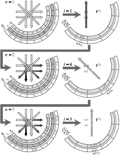
Looking at Fig. . , the question arises as to why f( ) is projected onto beam i = rather than onto i = . The chosen projection beam is, in fact, selected randomly and it is a popular strategy to implement the index as an equally distributed random variable.

As in Chap. , the ART mode of operation shall be clariﬁed by a speciﬁc example. Therefore, the example from Fig. . shall be consulted again. In summary, the following reconstruction procedure, which can be divided into four steps, is available as presented in Scheme . .

Scheme . Algebraic reconstruction technique (ART)

. Determination of an initial image:

f = ( , , , ) .

. Calculation of forward projections based on the nth estimation

p(n) = Af(n) .

. Correction of the estimation (projection index i being distributed randomly)

f(n)	=	f(n− )	−	"ai f(n− ) −T pi #				ai	T .
	=		−	ai	(	ai	)	(	)
					(		)

. Iteration from step when the method yields a change in consecutive image values larger than a ﬁxed threshold. Otherwise: End of iteration.

	6 Algebraic and Statistical Reconstruction Methods
	For the ﬁrst iteration, the result shall be written down explicitly here. In detail,
	and for the example from Fig. . , this means that one ﬁrst has to appoint the start
	image, f = ( , , , )T, before calculating the forward projections (being i =

Fig. . . The ﬁrst three algebraic reconstruction technique (ART) iterations of the exemplary

pixel image of Fig. . using f( ) = ( , , , )T as an initial image. The correct image values are f = ( , , , )T

6.3 Iterative Reconstruction with ART

here). Comparison with the measured projection yields the correction term and the ﬁrst approximation

f( )

−

!!		! .		( . )
	""		"
	""		"
	""		"
	""		"
	##		#

For instance in MatlabTM , the core content of the iteration can actually be programmed in only one line:

f = f − ((a(i, Y)>f − p(i)) (a(i, Y)>a(i, Y) )>a(i, Y) ) .

( . )

Figure . illustrates the interaction scheme for the ﬁrst three iterations using the exemplary pixel image of Fig. . . In the middle row, the second correction step (n = ), i.e., the result of ( . ), is shown. The second forward projection, p( ) = ( . , , , . , . , . ), has to be compared with the actual measured projections, p = ( , , , , , ), in order to determine the next correction terms that will further reﬁne the image. That way the di erences between the forward projections and the measured projections decrease in each iteration. In the last row of Fig. . , it can be seen that the correction terms have decreased signiﬁcantly after only three iterations.

Fig. . . Algebraic reconstruction technique convergence for the example from Fig. . . The pixel values are plotted versus the iteration steps from n = to n =

6 Algebraic and Statistical Reconstruction Methods

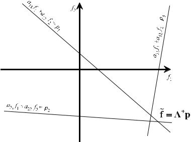
Fig. . . Search for the pseudo solution, $f = A+p, which represents a solution of the overdetermined system of equations in the least squares sense

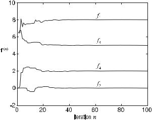
Figure . shows the convergence behavior in the pixel values of the image. The image values, f(n) = (f (n), f (n), f (n), f (n)), are plotted versus the iteration step, n. One can see that all image values converge very well. However, it should be mentioned that ART is noise-sensitive. The more the data are covered with noise, the worse the convergence behavior becomes (Dove ).

It is, incidentally, easy to understand that the system of equations ( . ) has exactly one solution: The intersection point of both straight projection lines. However, if only one more projection from another direction is added, usually it means that a clear intersection point cannot be found for real data as they are typically afﬂicted with noise and artifacts. Figure . illustratesXsuch a situation. In this case, and according to ( . ) to ( . ), a pseudo solution, f, in this over-determined system of equations must be found.

6.4

Pixel Basis Functions and Calculation of the System Matrix

Now that the principle of the ART has become clear, the next question has to be answered: Where can the system matrix, A, be obtained? In nuclear diagnostic imaging, the A entries are weights that are deﬁned by ( . ) and that reﬂect the actual contribution of every pixel to the activity. However, before the contribution of a pixel can be determined, the deﬁnition of a pixel that has been given in the introduction of this chapter should be brieﬂy discussed again here.

6.4 Pixel Basis Functions and Calculation of the System Matrix

6.4.1

Discretization of the Image: Pixels and Blobs

The discretization of an image can be described by a (linear) series expansion approach in which a continuous image is approximated with a linear combination of a ﬁnite number of basis functions. If f (x, y) = f (r) is the actual continuous spatial distribution of the attenuation coe cients, then the idea is to approximate the image f (r) with coe cients

in the sense that

f = (f , . . . , fN )T

( . )

(

)

(

−

) =

f j ϕj

( . )

j =

where N is the number of basis functions, ϕj(r), and attenuation coe cients, f j, with j = , . . . , N respectively. The vector r − rj is pointing from the center, rj, of basis function, j, to the current position, r. If the same basis function is used for every coe cient, the index, j, can be omitted. In imaging systems, the basis functions are usually aligned on a rectangular grid; however, hexagonal or other patterns are possible as well.

There are at least two factors that a ect the quality of the image approximation. The ﬁrst one is the number of basis functions that are used to represent an image. A high number of coe cients results in a better approximation than a low number of basis functions. In practice, however, the number of coe cients is often limited and chosen according to the resolution of the data. Additionally, the number of image coe cients also depends on the type of the chosen basis function. For example, for SPECT and PET applications it has been shown in (Yendiki and Fessler ) that blob-based reconstructions need fewer image coe cients for equal image quality than voxel-based reconstructions.

The second aspect, which a ects the image approximation, is the type of the basis function, ϕj(r). In general, basis functions can be categorized by the size of their spatial support, i.e., the size of the region of non-zero function values. While voxels, blobs, B-splines, and overlapping spheres have only small or local support, Fourier series are non-local or global basis functions.

In order to obtain reproducible results, it is necessary for the reconstructed image to be essentially independent of the orientation of the underlying grid. Therefore, basis functions that lead to shift and rotational invariance of the reconstruction should be preferred. Further, for X-ray CT, and some other imaging modalities, it is reasonable to constrain the image to non-negative values. Generally, it is su cient that if all image coe cients are positive, then the resulting function will be positive as well.

The most common basis functions in digital imaging are pixels and voxels for twoand three-dimensional cases respectively. Both are based on rectangular functions. An exemplary alternative representation, called the blob, is given by a local

6 Algebraic and Statistical Reconstruction Methods

basis function derived from a Kaiser–Bessel window introduced into the ﬁeld of

tomography by Lewitt ( , ). A blob is deﬁned as

− (

)

− (

)

−

\ =

(

) = /

m Jm

for

ϕjm,a,α

J α

otherwise

(

)

( . )

Fig. . . Basis functions of the image: a pixels, b blobs, and c proﬁle of the two di erent basis functions. The parameters for the blob shown here are a = , α = . , and m =

6.4 Pixel Basis Functions and Calculation of the System Matrix

where Jm is the modiﬁed Bessel function (Watson ) of order m; a is the radius of the basis function and α determines the shape of the blob. In contrast to pixels or voxels, blobs are rotationally ( D) or spherically ( D) symmetric basis functions. A two-dimensional comparison of pixels and blobs is shown in Fig. . , together with the function proﬁles through their centers.

Aligned on a simple quadratic grid, adjacent blobs must overlap in order to cover the entire image. However, due to their overlap, a reconstruction based on blobs is inherently smoother than a reconstruction using pixels or voxels. Hence, the change over from pixels to blobs adds a global smoothness to the reconstruction, without changing the underlying reconstruction algorithm.

6.4.2

Approximation of the System Matrix in the Case of Pixels

In Fig. . the nearest neighbors method for the determination of the weights, ai j, is presented for pixels schematically. The center of each pixel,

f j = fk N+l , ( . )

in the (N = n ) image shall have a quadratic neighborhood of the size b . T he index of the single projections runs from i = , . . . , M , whereas M = Np D stands for the

Fig. . . Determination of the weights, ai, j, with the nearest neighbors method. Here, the projection line is once again assumed to be a δ-line. However, this principle can be transferred easily to a line of the ﬁnite thickness, ξ. In contrast to Fig. . a ﬁner grid is determined here

6 Algebraic and Statistical Reconstruction Methods

total number of projections of the array detectors, d

, . . . , D

, and all projection

directions r

, . . . , Np

, which means that

pr D+d

( . )

holds true. The distance between the

beam, ξ

, and the pixel center can be deter-

mined by

ξd

xk cos

γr

yl sin

γr

( . )

Now, the following rule

results for the element a

i j: If(

))

− (

(

) +

cos(γr ) <

and ξ sin(γr )

( . )

then

ai j = ar D+d,k N+l = b .

( . )

Of course, higher order strategies are possible too. For instance, one may take the beam length through pixel (xk , yl ) (Toft ).

6.4.3

Approximation of the System Matrix in the Case of Blobs

The basis of tomographic imaging is the projection integral

pi = ∫ f (r)dη ( . )

where Li is a line segment between the source and detector pixel, i. T he integral represents the accumulated attenuation along a single beam if the width of the beam is inﬁnitely small. Substituting the deﬁnition of f (r) from ( . ) into ( . ) leads to

(

−

)

∫

f j ϕj

dη .

( . )

j =

Reordering integration and summation leads to

dηB f j

ϕj

(

−

)

( . )

j =

.L∫i

N .

0i j

a f

j =

where

ai j = ∫ ϕj(r − rj)dη

( . )

6.5 Maximum Likelihood Method

describes the contribution of the jth basis function to the ith beam. If pixels are used, then ai j is equal to the length of the intersection between beam i and pixel j as indicated in the subsection above. The coe cients ai j are not necessarily restricted to simple line integrals. It is also possible to formulate more realistic system models, which include, for instance, scatter and complex sampling trajectories. Furthermore, it has been discussed in (Müller ) that a ﬁnite beam width of the X-ray can easily be incorporated into the model as well.

6.5

Maximum Likelihood Method

In the previous iterative reconstruction methods, one always started with projections that could be modeled as line integrals. The maximum likelihood method gives an alternative description. It is a statistical estimation method in which the image obtained is one that matches the measured projection values best, taking into account the measurement statistics of the real values. For a brief overview of the measurement statistics in X-ray systems, Sect. . should be consulted.

Formulated more precisely, the measuring procedure must be modeled as a stochastic process whose parameters, f , have to be estimated through a given random sample, p (these are the projection values). In the following subsections it shall be distinguished whether the image reconstruction takes place for nuclear diagnostics (where f is the expectation value for the activity of the radioactive tracer) or for CT (where f is the expectation value for the attenuation of the X-ray quanta).

T his is a completely di erent approach to image reconstruction than the direct methods described above. It is typically used in situations where the number of quanta on the detectors is quite small and the sinogram therefore contains a lot of noise. In these cases, noise can dominate the reconstructed image if the direct methods for image reconstruction are used. Furthermore, the statistical method may be used even in situations where projections are either missing or inconsistent. These are cases in which the ﬁltered backprojection typically fails (Dempster ; Bouman and Sauer ).

As mentioned above, today, statistical methods are used in nuclear diagnostic imaging since PET and SPECT su er from much worse statistics than does CT. As the ﬁltered backprojection is faster than the iterative statistical methods and as the number of quanta is usually high in CT, there is no commercial push to transfer the iterative methods to the CT scanners of the current generation. However, this method must be presented here because, as with the continuously improving performance of computers, the iterative methods will, in the near future, also need a computing time that will be attractive for practical use. Additionally, statistical methods might possibly result in practical approaches that decrease the dose for CT. Low-dose imaging su ers from poor quantum statistics, such that statistical image reconstruction methods are appropriate.

6 Algebraic and Statistical Reconstruction Methods

6.5.1

Maximum Likelihood Method for Emission Tomography

The method presented by Shepp und Vardi ( ) is based on the assumption that the gamma quanta reaching the individual detector elements obey Poisson statistics. This is a direct consequence of the statistical properties of the radioactive de-

cay and it can be motivated according to the processes explained in

Sect. . .

The number of decays per time unit in the object pixel, f

j, represents

a Poisson-

distributed random variable with the expectation value f j .

Thus, the probability of measuring a certain number,

f j, of decays from

a pixel with an expected activity of f

can be modeled

through

f j

P(Nj = f j) =

*ffj j

e−f j .

( . )

Every linear combination

ai j f j

( . )

j =

of the N pixels with the expectation value

ai j f j

( . )

j =

is again Poisson-distributed and statistically independent, whereas the pixels are the statistically independent activities, f

of ( . ), the Poisson distribution	j, so that for the M projection values Mi = pi
		pi	pi		p
P(Mi = pi ) =		( pi)!		e−	i	( . )

holds true. One obtains the joint probability of all statistically independent projection values, that is, the probability of observing projection p at the given expectation value p , through multiplication of the single probabilities, so that

p p

) =

i =

(

pi)!

e−

( . )

(

holds true. By applying ( . ), one obtains

p p

j = ai j f j

e− j =

ai j

f j

p f

( . )

) = 1

)

(

pi !

(

i =

6.5 Maximum Likelihood Method

It does not make sense to understand ( . ) as a function of the ﬁxed projection measurement, p. Rather, ( . ) is given as a function of the variable parameter f , i.e., the expectation value of the spatial activity distribution

				N		pi
				N
						N
L	(	f	M	j = ai j f j		e− j = ai j f j .	( . )
	(		) = 1		pi !
			7		pi !
			i =

( . ) is the likelihood function. The key idea of the maximum likelihood method is to vary the expectation values of all activities, f j , with j = , . . . , N in order to ﬁnd the maximum of the likelihood functional, L. The distribution f , for which L is maximal, is called the maximum likelihood solution of the statistical reconstruction problem and reﬂects the most probable solution.

Through the logarithm of L, ( . ) simpliﬁes to

(

) =

(

# −

(

)) =

pi !

) −

( . )

i =

pi ln j =

ai j f j !

j =

ai j f j ! .

l(f ) is called the log likelihood function. Taking the logarithm is possible since the logarithm is a strictly monotonous function and, therefore, the location of the maximum will not change. Thus, the optimization can formally be expressed by

f = max l(f ) , ( . )

max f Ω

where Ω is set of possible solutions. A necessary condition for the maximum of l(f ) is the vanishing of the ﬁrst derivation

∂l

pi ∂ ln

air !

(

)

j = ai j f j

−

∂ fr

i =

∂ fr

pi air

air

pi air

air .

−

= j =

" = j =

i =

ai j f j

i =

ai j f j

i =

That means that, overall, the expression

∂l f

p air

−

∂(fr )

i =

iai j f

i = air

( . )

has to result in zero.

However, a su cient condition for a global maximum is the concavity of the function that is to be maximized. This condition is usually veriﬁed with the second

6 Algebraic and Statistical Reconstruction Methods

derivative, which means application of the Hessian matrix with respect to the f j with j = , . . . , N ,

∂

−

∂ l

(

)

j = ai j f j

7∂ fs

∂ fr ∂ fs

i = pi air

( . )

−

pi air

ais

= −

pi air ais

ai j f j

The symmetric Hessian matrix is negative semi-deﬁnite, i.e., l(f ) is concave and the optimal value obtained is a global maximum. As a consequence, the commonly referred to Kuhn–Tucker conditions for each j are fulﬁlled too (Shepp and Yardi), i.e., it holds true that

∂l

f j

∂ f j

fmax

for all j with

f j

( . )

and

(

)

∂l

for all j with f j

( . )

∂ f j

)

fmax

(

The ﬁrst Kuhn–Tucker conditionH

assures

that

the

activity

values

f j with j

, . . . , N

cannot become negative and, at the same time, it leads to an iteration

scheme that will be derived in the following.

If ( . ) is applied to ( . ), one obtains

∂l f

pi air

air

( . )

i =

∂ fr

i =

( ) =

ai j f j

−

thus

pi air

air

( . )

i =

ai j f j −

i =

and, therefore,

pi air

( . )

i =

ai j f j

= i

air

6.5 Maximum Likelihood Method

Obviously, the intersection point between a straight line of slope one and the functional on the right side of ( . ) must be found. The intersection point is obtained by the ﬁxpoint iteration,

(n+ )

fr (n)

pi air

( . )

(n)

= i

air

ai j f j

which, at the same time, represents the iteration rule for the image reconstruction. ( . ) is called the Expectation Maximation (EM) algorithm. The idea is to assume fr (n+ ) as the reﬁned value for the activity at pixel r for every step n n + . In a forward projection

	N
pi (n)	=	ai j f j (n) ,	( . )
	j =

the expected projection values on the detector elements resulting from this are then calculated in the denominator of ( . ). These estimates are compared with the actual measured projection values, pi . The resultant multiplicative correction factor

				M			pi air	( . )
							pi air
7					7
	M		i	=		N	(n)
i		air		=			ai j f j
i	=	air	j			=	ai j f j
	=					=

for activity values fr (n) in all pixels, leads to a new and improved image, fr (n+ ),

with r

, . . . , N

. The log likelihood function ( . ) increases with each step

and a maximum is found within a given uncertainty, if the iterative re-

n =

)

(

)

ﬁnement step f (

falls below a given threshold.

For initialization

of−the iteration,

the average projection sum

f j ( )

pi , for all j

, . . . , N

( . )

M i =

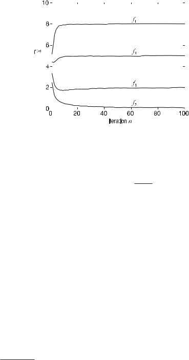
turns out to be convenient. Figure . demonstrates the convergence for the example from Fig. . . ( . ) represents a simple gradient method (Lange et al. ). This can be seen when adding a zero to the right side of ( . ), thus

fr (n)

- M

pi air

fr (

)

fr (

)

.i =

air .

( . )

+ i

air

ai j f

(n)

i =

/ j

−

	6 Algebraic and Statistical Reconstruction Methods

Fig. . . Convergence of the maximum likelihood method for the example from Fig. . . The single pixel values are shown in the iteration steps n = to n =

in which the term in brackets is just equal to ( . ), meaning that

or in vector notation

Therefore,

	fr (n)		∂l f
fr (n+ ) = fr (n) +		&	∂(fr )	' ,
	iM air
7
=

(n+ ) = f (n) + D f (n) grad (l(f )) .

					M		"
D f	(n)	) =	diag		fr (n)		!

(				i =			"
					7	air	#
							"

( . )

is a diagonal matrix.

Contrary to iteration ( . ), no negative pixel values occur during iteration here. Scheme . once again summarizes the individual steps that are to be implemented for realization. This overview clariﬁes that the cost is deﬁnitely higher than that of ﬁltered backprojection.

The most important properties of the maximum likelihood method resulting from the iteration formula ( . ) are:

The grad operator is deﬁned as a column vector here.

6.5 Maximum Likelihood Method

Scheme . Maximum likelihood method in nuclear diagnostics

. Determination of a start image that is an initial estimation:

( )

f j

pi , for all j

, . . . , N .

. Determination of a normalization:

air .

. Calculation of forward projections based on the (n − )th estimation:

p = Af(n− ) .

. Calculation of the relative di erence between the measured projection, pi , and the

forward projection based on the (n − )th estimation:

rel

. Backprojection of the relative di erence of the projections into the image space:

fback = ATprel .

For every pixel, the current estimation

is multiplied with the backprojection

. of the relative di erence and weighted

(with− )the normalization from step :

(n− ) back

fr(n) =

. Go on with step as long as the method comes up with di erences larger than a chosen threshold in further iterations. Otherwise: End of iteration.

•	Positivity, i.e., it holds true that	f j (n)		( . )
•	for all pixels j and all iteration steps n, if f:j ( )		:	.
•	The algorithm is scaling, i.e.,
	The algorithm is scaling, i.e.,

ai j f j (n)

f j (n)

ai j

pi (n)

i =

j =

i =

holds true for all iteration steps n

•

Monotonous maximization of L(f ), i.e.,

(

)

L f

(

(n+ )

) :

f (n)

whereas the identity is only true for L

(

f (n)

) = f Ω

(

)

max

( . )

6 Algebraic and Statistical Reconstruction Methods
6.5.2
Maximum Likelihood Method for Transmission CT
In transmission CT, the projection sum ( . ) cannot be measured directly because
one does not deal with gamma quanta originating inside the body. The raw data,
rather, are the X-ray quanta that are generated in the X-ray tube outside the body,
attenuated exponentially when passing through the body. As shown in				Sect. . . ,
the number of quanta generated in the X-ray tube is a Poisson-			distributed random

variable. Discussing the absorption or the scattering processes of X-ray quanta in
a pixel, j, as random events, the number of quanta reaching the detector after pass-
ing through the pixel per time unit obeys Poisson statistics as well.
The probability of an absorption and scattering process is proportional to the
attenuation coe cient, f j, which means that the attenuation of the intensity caused
by pixel j – provided there is a constant X-ray path length – is given by
	I	−f j .		( . )
	I	−f j .		( . )

As in the previous section, it is again the absolute number of quanta measured by the detector that shows a Poisson distribution.

Based on the Beer–Lambert law of attenuation and the fact that the number of X-ray quanta is proportional to the radiation intensity, one can write

	N	a		f
Ii ni = n e	−		i j
					j	( . )
	j =				.

The number of quanta, n , generated by the X-ray tube is constant and can be assumed to be known through calibration. f j are the expectation values of the attenuation coe cients. In contrast to the section above, one has to formulate the maximum likelihood problem that is to be solved for transmission CT or, more speciﬁcally, for the number of X-ray quanta in detector i, i.e., ni , and not directly for the image value, f j . The probability of measuring a certain number, ni , at an expected value for the quanta number, ni , can be modeled as

	ni	ni		n
P(ni ) =	( ni)!		e−		i	( . )

where all ni are again considered to be statistically independent.

One obtains the joint probability of all measured, statistically independent numbers for X-ray quanta, i.e., the probability of observing the set of numbers, n, at

In Sect. . . it has been shown that cascaded Poisson processes again obey a Poisson distribution.

6.5 Maximum Likelihood Method

the given expectation value, n , through multiplication of the single probabilities, so that

	(		M	ni	ni	n
			) = 1
P				( ni)!		e− i	( . )
		n n	i =

holds true. By applying ( . ), one obtains

−

i j

e j =

a i j f

(

− j

(

)

) = 1

e−n e =

n n

n f

( . )

i =

ni !

Since the number of measured X-ray quanta, n, is not a variable, ( . ) should instead be understood as a function of the variable distribution of the expectation values of attenuation coe cients, f , i.e.,

				N		ni
			M	n e− j = ai j f j !
L		f			"
L	(	f	) = 1	ni !	#
	(		) = 1
			i =

	N	a i j f	j
	−		j
e−n e	j =
e−n e	j =		.	( . )

( . ) is the likelihood function for transmission CT (Andia ). Here, analogous to the previous section, the key idea of the maximum likelihood method is the variation of the expectation values of attenuation coe cients to ﬁnd the optimal likelihood functional, L. Again, the distribution f , for which L is a maximum, is called the maximum likelihood solution of the statistical reconstruction problem and reﬂects the most probable solution.

The logarithm of L simpliﬁes ( . ) to

l(f ) = ln (L(f ))

M		N	ai j

=
	ln	n e− j =

=ni ln(n ) − ni

f j !	ni						N	ai j f j !
f j !	ln ni !			) −	n e− j =			ai j f j !		( . )
"	− (			) −					"	( . )
#									#
j N ai j f j			ln ni !					N	ai j f j ! .
j N ai j f j		−	ln ni !			) −	n e− j =		ai j f j ! .
		−		(		) −			"
=									#
=

6 Algebraic and Statistical Reconstruction Methods

l(f ) is the log likelihood function of transmission CT. Formally, one may write the optimization as

f		max	l	(	f	)	,	( . )
	max = f Ω			(		)

where Ω denotes the set of possible solutions. A necessary condition for the maximum of l(f ) is the vanishing of the ﬁrst derivation

ni ln

ai j f

∂l

∂

(

) −

ni j = ai j f j

ln ni !

) −

n e− j =

(

)

− (

∂ fr

i =

j N ai j f j

f j !

∂ ni

∂

n e− j = ai j

−

∂ fr

# N

i M

ni air

f j !

n air e− j = ai j

iM air e− j = ai j

−

This means that the expression

∂l	f		M	N	a f		M
		=		−
					i j	j	−
∂(fr )			n i = air e j =				i = ni air

f j	M
	−	ni air .
	i =	( . )
		( . )
		( . )

has to become zero again.

However, the su cient condition for a global maximum of l f is the concavity

of the function that is to be maximized. This condition is usually veriﬁed with the

second derivative. That means in the case of f

(

)

of the Hessian matrix is

with j = , . . . , N , the application

∂

n air e− j =

i j

−

ni air

∂ f ∂ f

∂ f

(

)

( . )

ai j f j

# M

ai j f j

! .

n air e− j =

ais

n i

ais air e− j =

(− )"

= −

6.5 Maximum Likelihood Method

Here, too, the symmetric Hessian matrix is negative semi-deﬁnite, i.e., l(f ) is concave and the optimal value obtained is a global maximum. As a consequence, the Kuhn–Tucker conditions for each j are fulﬁlled, too, which again leads to an iteration scheme. When applying ( . ) to ( . ), one obtains

(

)

fr ∂l∂ ffr

ni air

( . )

i j j

−

thus

−

fr n

i j

i =

air e

j =

i =

ni air

( . )

and ﬁnally

f n

i j

−

air e

j =

( . )

= i

i =

ni air

Obviously, the intersection point between a straight line of a slope of one and the functional on the right side of ( . ) must be found. The intersection point is obtained by the ﬁxpoint iteration

(n)

ai j f

(n)

−

(n+ )

air e j =

( . )

i =

= i

ni air

which also represents the iteration rule for image reconstruction. Recalling that the number, ni , of X-ray quanta measured in the detector, i, is proportional to the intensity of the X-ray radiation,

								N
							− ai j f j
one may write ( . ) as			ni = n e					j =		( . )
								N
							M	− ai j f j (n)
fr (	n	+	) = fr (	n	)	7		air e j =	.	( . )
fr (		+	) = fr (		)	7		iM air e−pi	.	( . )
							i =
								7
								=
However, according to Beer–Lambert’s law, the measured projection values,
				=			N
			pi	=				ai j f j ,		( . )
			pi					ai j f j ,		( . )

j =

6 Algebraic and Statistical Reconstruction Methods

appear as an argument of the exponential function in the denominator of ( . ).

(n+ )

In ( . ), fr is the reﬁned value for the X-ray attenuation at pixel r for every step n n + . From this, the number of expected X-ray quanta,

			N
n(	n	)	− ai j f j (n)	,	( . )
n(		)	e j =	,	( . )
i

measured by the detectors can be determined. These are compared with the actual measured X-ray quanta,

		ni e−pi		.		( . )
The ratio
		N
M		− ai j f j (n)		M
	air e	j =	_		air e−pi	( . )
i=				i =

of ( . ) improves the image in every iteration. The log likelihood function ( . )

increases with each step n		n and a maximum is found within a given uncer-
tainty if the iterative	reﬁnement step, f		(n+ )		(n)	, falls below a given thresh-
		+	r	−	fr
old.
In order to write ( . ) in the form
	f (n+ ) = f (n) + D(f (n))grad (l(f ))						( . )

just as in the previous section, the diagonal matrix ( . ) of the emission tomography has to be replaced by the appropriate expression for transmission CT:

D f

(n)

)

diag

fr (n)

! .

(

i =

air e−pi

As shown by (Lange and Fessler ), ( . ) can be written#

fr (n)

∂l

fr (n+ ) = fr (n) +

∂(fr )

air e−pi

)

- M

fr (n)

fr (

air e− j = ai j f j (

)

air e−p

+ i

−

air e−pi

i =

.i =

( . )

i	B .	( . )
	.
	C
	.
	D

Unfortunately, the simple ﬁxpoint iteration ( . ) is often numerically unstable. Therefore, methods for regularization of the inverse problem have to be used. These methods shall be presented brieﬂy in the next section.

The grad operator is deﬁned as a column vector here.

6.5 Maximum Likelihood Method

6.5.3

Regularization of the Inverse Problem

The maximum likelihood approach ( . ) in imaging is a very high dimensional inverse problem and is often revealed to be unstable, i.e., it may produce oscillations that complicate the search for optimal parameters, f . T he typical countermeasure to this problem is the introduction of a regularization term to the log likelihood function. This penalty term controls the compromise between spatial resolution and noise in the image. It should be noted here that this compromise has to be found for the method of the ﬁltered backprojection as well: In ﬁltered backprojection one has to ﬁnd an appropriate deviation from the linear weighting of the spectrum of the projection integral in order to attenuate high frequencies. This regularization deﬁnitely reduces noise in the image; however, at the same time this is also true for the spatial resolution. This is a typical trade-o in ill-posed problems.

In terms of linear algebra, regularization improves the conditioning of the inverse problem, which potentially leads to faster convergence of the algorithm. Furthermore, it is possible to integrate a priori known, desired properties of the image into the regularization strategy.

The estimation of the image for the regularized problem is formally given as an

additive extension of ( . ), i.e.,

max

(

)) +

ln R

(

))

( . )

max = f Ω

(

where R represents the regularization functional and Ω denotes the set of possible solutions, which is, compared with ( . ), limited by the penalty term, R. Severe complications of this method are that one has to ﬁnd an appropriate regularization functional, R, and a parameter that controls the strength of the penalty.

Bayes’ view, which understands the regularization as an a priori model, shall brieﬂy be described here. A typical Bayesian estimation method is the maximum a posteriori (MAP) method. For this method, two statistical models are required. One model describes the physical process of emission of gamma quanta (for emission CT), which means

	N	ai j f j !
pi obeys Poisson	j =	ai j f j !	,	( . )
		#
or the transmission of X-ray quanta (in transmission CT), which means
		N	"
			"	( . )
ni obeys Poisson n e− j = ai j f j			! .	( . )
			#

This ﬁrst model is the original maximum likelihood term.

The other model, namely the a priori model, is the probability distribution of the original image. The reconstruction quality of the MAP method depends sensitively

6 Algebraic and Statistical Reconstruction Methods

on the choice of an appropriate second model. T he choice of thea priori model seems to be a big challenge, since detailed knowledge about the image that is to be reconstructed is required and has to be formulated mathematically as the functional R(f ), called the prior, in ( . ). Fortunately, it can be shown (Green ) that knowledge is neither necessary on a large scale nor does one need complex knowledge about the image involved to obtain su cient regularization. In order to suppress noise in the reconstructed image, it is reasonable to require that gray values of spatially neighboring pixels do not di er substantially in their mean. The a priori knowledge is hence limited to the direct neighborhood and can be formulated in a simple mathematical form.

In practice the image is very often modeled as a Marko random ﬁeld (MRF). For such stochastic processes, the conditional distribution, P(fn f , . . . , fn− ), only depends on the gray values of direct neighboring pixels . Therefore, an important expression is the Gibbs distribution

	(		) = Z	−λq Vc (f )
R		f		−λq Vc (f )
R		f		e c C	,	( . )

because a random ﬁeld is a Marko random ﬁeld if, and only if, the probability distribution obeys function ( . ). Z is a normalizing constant , Vc(f ) is a potential function of a local group of pixels, c is commonly called a clique, and C denotes the set of all cliques (Lehmann et al. ). Examples of the possible cliques of a - and-neighborhood in a two-dimensional image are given in Fig. . .

The parameter λq represents the regularization parameter (the control factor for the inﬂuence of regularization) where q . In Andia ( ) several potential functions are given. A very simple function for q = is the potential

Fig. . . The cliques of a - and -neighborhood for the deﬁnition of Gibbs potential

In so far as the Marko process is the stochastic equivalent to the di erential equation (Lehmann et al. ).

In physics Z is called the partition function.In physics λ−q represents the temperature.

6.5 Maximum Likelihood Method

that penalizes the squares of the di erence of neighboring pixels d	= (	f	i	−	f	j)	,
thus	= (		i	−		j)
Vck (d) = d .				( . )

This potential, the commonly referred to Gaussian MRF, suppresses the noise, but also penalizes edges in the image. In order to be able to control the strength of the regularization, one deﬁnes

R	f		−λq	w j,k f j −fk q
R	f		e	j,k C	( . )

( ) = Z

as the Gibbs distribution of the generalized Gaussian MRF (GGMRF; Bouman and

Sauer ). Here, wj,k is a weighting that assesses the respective neighborhood of the clique (e.g., wj,k = for orthogonal neighbors and wj,k = − for diagonal neighbors [Green ]). Additionally, smaller values of the exponent, q, of the potential function of ( . ) allow sharper edges within the image reconstruction.

Of course one can also ﬁnd edge preserving regularizations by an appropriate choice of the potential function. The regularized log likelihood function for transmission CT that results from ( . ) reads

	iM			jN	ai j f j		N
l f	iM		ni	jN	ai j f j		n e− j = ai j f j !	ln R f ,	( . )
X	=	−		=		−	"	+ ( )
(	) =	−				−	"	+ ( )
							#

whereas the partition function, Z, which depends on the regularization parameter, λq , does not have to be considered for optimization (Hebert and Leahy ). An iterative ﬁxpoint solution can be found for ( . ) as well. Using the recipe of the section above, starting with ( . ), one obtains

f j !

∂l f

∂

ai j f j

∂

n e− j = ai j

∂ ln R

∂ f

X r

)

(

−

(

( . )

∂ λ

air e− j = ai j f j

air

j,k C wj,k Sf j − fk S

and ﬁnally=

i =

−

∂ f

−

− ai j f j(n)

i =

air e j =

fr(

)

fr(

)

air e−pi

C wk j

f j

q−

sign fk

f j

, ( . )

λq q ci

−

for the special GGMRF approach of ( . ).

6 Algebraic and Statistical Reconstruction Methods

6.5.4

Approximation Through Weighted Least Squares

Another method of stabilizing the optimization is to incorporate the reliability of the measured values. This is possible with the method of weighted least squares for which the functional


fmin	min		Af p TC− Af p		( . )

	f	Ω	),( and−where)	Ω(denotes− )Othe set of possible so-
has to be minimized (Andia=		M

lutions. Contrary to ( . ), the inverse covariance matrix, C− , which weights the measured values of low reliability adequately, is incorporated here.

The functional ( . ) that has to be optimized results from a Taylor expansion of the log maximum likelihood functional

ni ln n

l f

ai j f j ln ni !

n e− j = ai j f j !

(

) =

( ) −

− ( ) −

( . )

ni ln n

ln ni !

n e

−pi

i =

( ) −

− ( ) −

in which the expressions for the expected projection sums,

ai j f j ,

( . )

j =

are used and the dependencies of pi

( . )

Bouman ), hence

are developed to the second order (Sauer= andi

l f

ni ln n

ni pi

ln ni !

i =

( )

( ) −

− ( − pi

) − ( )

n e−pi

e−pi

e−

pi pi

−

( − ) +

( − )

−

ln n

ni pi

ln ni !

pi pi

i =

( ) −

− ( ) − + ( − ) − ( − )

ln n

ln ni !

ni pi

i =

( ) − ( ) − −

− ( − )

ln n

ln ni !

i =

( ) − ( ) −M ( + ) −

( − )

ni pi

ni ln n

ln ni !

pi .

i =

= −

( − ) +

(

( ) − ( ) − ( + ))

( . )

6.5 Maximum Likelihood Method

Overall, this expression can be summarized as

(

) −

−

(

)

( . )

i =

j = ai j f j

! !

i =

or, equivalently, in vector and matrix form as

# #

l(f ) −

(Af − p)TC− (Af − p) + c (n)

( . )

so that the maximization of the log likelihood function ( . ) can be approximated by the minimization of the weighted least squares in ( . ). Therefor, c(n) is independent of f and can be ignored in the optimization. This result holds analogously true for the maximum likelihood approach for emission CT.

Finally, the physical meaning of the covariance matrix should be explained. In the case of emission CT,

		p		n			( . )
is the number of quanta that is measuredi =in ithe detector and
		n				"
			n			"
			n	. .	.	!
C				. .	.	!	( . )
	=		. .		.	"
						"
			. .			#
			. .		nM "

is the covariance matrix. ( . ) is the central statement for the Poisson distribution of detected quanta, namely σi = `ni a.

In the case of transmission CT, it holds true that

					n
		pi = ln
		pi = ln			ni
and	n						!
	n						!

							"
							"
							"
			n				"
	=			. . .			"
C				. . .			"
C				. . .			" .
						nM	"
				.	.		"
				.	.		"
							#

( . )

( . ) implies that σi = `ni a. This means that the more quanta that are measured, the smaller the signal variance and, consequently, the stronger the data are

6 Algebraic and Statistical Reconstruction Methods

weighted as reliable within the minimization (in Chap. this circumstance will

be discussed in detail). The reverse holds for emission CT. The approximated regu-

larized maximum likelihood approach then reads

min

p TC−

λq

( . )

j,k

min

j,k C

(

− )

(

− ) +

S − S

and can be optimized with, for example, the Newton–Raphson method (Fessler; Bouman and Sauer ).

<<< < Предыдущая 1 23 / 73 4 5 6 7 > Следующая >>>

Соседние файлы в предмете [НЕСОРТИРОВАННОЕ]

#
25.04.201979.36 Кб1Boiler_and_reactor_building_Unit4.doc
#
29.05.201519.47 Кб32Brass.docx
#
29.05.201526.89 Кб22Buddizm.docx
#
29.05.20151.2 Mб34Bukhgaltersky_uchet_UP_2012.doc
#
29.05.20156.06 Mб3107BusinessEnglish_Nikolaenko.pdf
#
29.05.201515.29 Mб42Buzug_Computed_tomography_From_photon_stat.pdf
#
29.05.2015403.08 Кб23BZhD_otvety-1.pdf
#
17.09.2019822.27 Кб11bzhd_otvety.doc
#
23.11.2019302.59 Кб6b_12101809_t_k_r_fizika.doc
#
25.08.20191.49 Mб69C2.doc
#
29.05.20151.42 Mб27CFZ_TREBOVANIYa.doc