B.Thide - Electromagnetic Field Theory

(one equation for and one equation for each of the three components of A). Each of these four scalar equations is an inhomogeneous wave equation of the following generic form:

where is a shorthand for either or one of the vector components of A, and f is the pertinent generic source component.

We assume that our sources are well-behaved enough in time t so that the Fourier transform pair for the generic source function

Inserting the Fourier representations (3.20a) and (3.21a) into Equation (3.19) above, and using the vacuum dispersion relation for electromagnetic waves

the generic 3D inhomogeneous wave equation, Equation (3.19), turns into

which is a 3D inhomogeneous time-independent wave equation, often called the 3D inhomogeneous Helmholtz equation.

As postulated by Huygen's principle, each point on a wave front acts as a point source for spherical waves which form a new wave from a superposition of the individual waves from each of the point sources on the old wave front. The solution of (3.23) can therefore be expressed as a superposition of solutions of an equation where the source term has been replaced by a point source:

i

and the solution of Equation (3.23) on the previous page which corresponds to the frequency ! is given by the superposition

Z

!(x) = d3x0 f!(x0)G(x;x0) (3.25)

V0

The function G(x;x0) is called the Green function or the propagator.

In Equation (3.24) on the preceding page, the Dirac generalised function(x x0), which represents the point source, depends only on x x0 and there is no angular dependence in the equation. Hence, the solution can only be dependent on r =jx x0j and not on the direction of x x0. If we interpret r as the radial coordinate in a spherically polar coordinate system, and recall the expression for the Laplace operator in such a coordinate system, Equation (3.24) on the previous page becomes

Away from r = jx x0j = 0, i.e., away from the source point x0, this equation takes the form

where C are constants.

In order to evaluate the constants C , we insert the general solution, Equation (3.28), into Equation (3.24) on the previous page and integrate over a small

The volume integrated Equation (3.24) on the preceding page can under this assumption be approximated by

Z

=d3x0 ( x x0 )

V0

i

In virtue of the fact that the volume element d3x0 in spherical polar coordinates is proportional to jx x0j2, the second integral vanishes when jx x0j ! 0. Furthermore, from Equation (M.86) on page 185, we find that the integrand in the first integral can be written as 4 (jx x0j) and, hence, that

Insertion of the general solution Equation (3.28) on the preceding page into Equation (3.25) on the facing page gives

The Fourier transform to ordinary t domain of this is obtained by inserting the above expression for !(x) into Equation (3.21a) on page 43:

If we introduce the retarded time tret0 and the advanced time tadv0 in the following way [using the fact that in vacuum k=!=1=c, according to Equation (3.22) on page 43]:

This is a solution to the generic inhomogeneous wave equation for the potential components Equation (3.19) on page 43. We note that the solution at time t at the field point x is dependent on the behaviour at other times t0 of the source at x0 and that both retarded and advanced t0 are mathematically acceptable solutions. However, if we assume that causality requires that the potential at

(t;x) is set up by the source at an earlier time, i.e., at (tret0 ;x0), we must in Equation (3.35) above set C = 0 and therefore, according to Equation (3.31),

C+ = 1=(4 ).

i

The retarded potentials

From the above discussion on the solution of the inhomogeneous wave equation we conclude that, under the assumption of causality, the electrodynamic potentials in vacuum can be written

Since these retarded potentials were obtained as solutions to the Lorentz equations (3.14) on page 41 they are valid in the Lorentz gauge but may be gauge transformed according to the scheme described in subsection 3.3.1 on page 41. As they stand, we shall use them frequently in the following.

EXAMPLE 3.1 BELECTROMAGNETODYNAMIC POTENTIALS

In Dirac's symmetrised form of electrodynamics (electromagnetodynamics), Maxwell's equations are replaced by [see also Equations (1.50) on page 17]:

In this theory, one derives the inhomogeneous wave equations for the usual “electric” scalar and vector potentials ( e;Ae) and their “magnetic” counterparts ( m;Am) by assuming that the potentials are related to the fields in the following symmetrised form:

In the absence of magnetic charges, or, equivalenty for m 0 and Am 0, these formulae reduce to the usual Maxwell theory Formula (3.10) on page 39 and Formula (3.6) on page 38, respectively, as they should.

Inserting the symmetrised expressions (3.38) into Equations (3.37) above, one obtains [cf., Equations (3.11) on page 39]

i

By choosing the conditions on the vector potentials according to Lorentz' prescripton [cf., Equation (3.13) on page 40]

exhibiting once again, the striking properties of Dirac's symmetrised Maxwell theory.

END OF EXAMPLE 3.1C

Bibliography

[1]L. D. FADEEV AND A. A. SLAVNOV, Gauge Fields: Introduction to Quantum Theory, No. 50 in Frontiers in Physics: A Lecture Note and Reprint Series. Benjamin/Cummings Publishing Company, Inc., Reading, MA . . . , 1980, ISBN 0- 8053-9016-2.

[2]M. GUIDRY, Gauge Field Theories: An Introduction with Applications, John Wiley & Sons, Inc., New York, NY . . . , 1991, ISBN 0-471-63117-5.

[3]J. D. JACKSON, Classical Electrodynamics, third ed., John Wiley & Sons, Inc., New York, NY . . . , 1999, ISBN 0-471-30932-X.

[4]L. LORENZ, Philosophical Magazine (1867), pp. 287–301.

i

[5]W. K. H. PANOFSKY AND M. PHILLIPS, Classical Electricity and Magnetism, second ed., Addison-Wesley Publishing Company, Inc., Reading, MA . . . , 1962, ISBN 0-201-05702-6.

i

4

Relativistic Electrodynamics

We saw in Chapter 3 how the derivation of the electrodynamic potentials led, in a most natural way, to the introduction of a characteristic, finite speed of propagation in vacuum that equals the speed of light c = 1=p"0 0 and which can be considered as a constant of nature. To take this finite speed of propagation of information into account, and to ensure that our laws of physics be independent of any specific coordinate frame, requires a treatment of electrodynamics in a relativistically covariant (coordinate independent) form. This is the object of this chapter.

4.1 The Special Theory of Relativity

An inertial system, or inertial reference frame, is a system of reference, or rigid coordinate system, in which the law of inertia (Galileo's law, Newton's first law) holds. In other words, an inertial system is a system in which free bodies move uniformly and do not experience any acceleration. The special theory of relativity1 describes how physical processes are interrelated when observed in different inertial systems in uniform, rectilinear motion relative to each other and is based on two postulates:

1The Special Theory of Relativity, by the American physicist and philosopher David Bohm, opens with the following paragraph [4]:

“The theory of relativity is not merely a scientific development of great importance in its own right. It is even more significant as the first stage of a radical change in our basic concepts, which began in physics, and which is spreading into other fields of science, and indeed, even into a great deal of thinking outside of science. For as is well known, the modern trend is away from the notion of sure `absolute' truth, (i.e., one which holds independently of all conditions, contexts, degrees, and types of approximation etc..) and toward the idea that a given concept has significance only in relation to suitable broader forms of reference, within which that concept can be given its full meaning.”

49

i

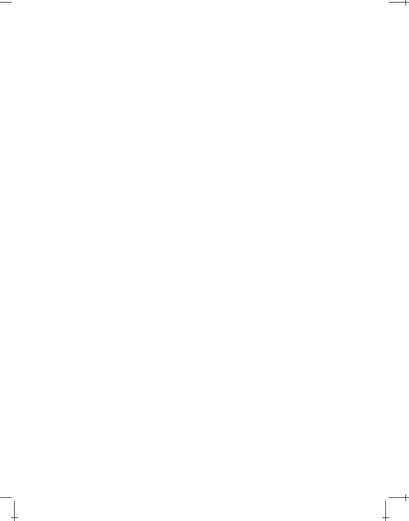
FIGURE 4.1: Two inertial systems and 0 in relative motion with velocity v along the x = x0 axis. At time t =t0 =0 the origin O0 of 0 coincided with the origin O of . At time t, the inertial system 0 has been translated a distance vt along the x axis in . An event represented by P(t;x;y;z) inis represented by P(t0;x0;y0;z0) in 0.

Postulate 4.1 (Relativity principle; Poincaré, 1905). All laws of physics (except the laws of gravitation) are independent of the uniform translational motion of the system on which they operate.

Postulate 4.2 (Einstein, 1905). The velocity of light in empty space is independent of the motion of the source that emits the light.

A consequence of the first postulate is that all geometrical objects (vectors, tensors) in an equation describing a physical process must transform in a covariant manner, i.e., in the same way.

4.1.1 The Lorentz transformation

Let us consider two three-dimensional inertial systems and 0 in vacuum which are in rectilinear motion relative to each other in such a way that 0 moves with constant velocity v along the x axis of the system. The times and the spatial coordinates as measured in the two systems are t and (x;y;z), and t0 and (x0;y0;z0), respectively. At time t = t0 = 0 the origins O and O0 and the x and x0 axes of the two inertial systems coincide and at a later time t they have the relative location as depicted in Figure 4.1.

i

where v = jvj. In the following, we shall make frequent use of these shorthand notations.

As shown by Einstein, the two postulates of special relativity require that the spatial coordinates and times as measured by an observer in and 0, respectively, are connected by the following transformation:

Taking the difference between the square of (4.3a) and the square of (4.3b) we find that

From Equations (4.3) above we see that the y and z coordinates are unaffected by the translational motion of the inertial system 0 along the x axis of system. Using this fact, we find that we can generalise the result in Equation (4.4) to

which means that if a light wave is transmitted from the coinciding origins O and O0 at time t = t0 = 0 it will arrive at an observer at (x;y;z) at time t in and an observer at (x0;y0;z0) at time t0 in 0 in such a way that both observers conclude that the speed (spatial distance divided by time) of light in vacuum is c. Hence, the speed of light in and 0 is the same. A linear coordinate transformation which has this property is called a (homogeneous) Lorentz transformation.

4.1.2 Lorentz space

Let us introduce an ordered quadruple of real numbers, enumerated with the help of upper indices = 0;1;2;3, where the zeroth component is ct (c is the

i

speed of light and t is time), and the remaining components are the components of the ordinary R3 radius vector x defined in Equation (M.1) on page 170:

We want to interpret this quadruple x as (the component form of) a radius four-vector in a real, linear, four-dimensional vector space.1 We require that this four-dimensional space be a Riemannian space, i.e., a space where a “distance” and a scalar product are defined. In this space we therefore define a metric tensor, also known as the fundamental tensor, which we denote by g .

Radius four-vector in contravariant and covariant form

The radius four-vector x =(x0;x1;x2;x3) =(ct;x), as defined in Equation (4.6), is, by definition, the prototype of a contravariant vector (or, more accurately, a vector in contravariant component form). To every such vector there exists a dual vector. The vector dual to x is the covariant vector x , obtained as (the upper index in x is summed over and is therefore a dummy index and may be replaced by another dummy index ):

This summation process is an example of index contraction and is often referred to as index lowering.

Scalar product and norm

The scalar product of x with itself in a Riemannian space is defined as

This scalar product acts as an invariant “distance,” or norm, in this space.

If we want the Lorentz transformation invariance, described by Equation (4.5) on the previous page, to be the manifestation of the conservation

1The British mathematician and philosopher Alfred North Whitehead writes in his book The Concept of Nature [13]:

“I regret that it has been necessary for me in this lecture to administer a large dose of four-dimensional geometry. I do not apologise, because I am really not responsible for the fact that nature in its most fundamental aspect is fourdimensional. Things are what they are. . . ”

i