CLICK ON Exit

When asked if you want to save the changes

SELECT No

GPSS World will close without saving the open GPSS World Objects.

Lesson 2 - Running a Simulation

In this lesson, we will study a small simulation. GPSS World has many interactive features which we will defer to later lessons. For now, we will be content to restrict ourselves to running a "classic" sample simulation, the barber shop.

Before we begin, we need to go over a few basic definitions. A GPSS World Model Object is defined to be a sequence of Model Statements. When you know what a Model Statement is, you will know how to build models.

A Model Statement is either a Block Statement, a Command, or a PLUS Procedure Statement. That’s all there is to it. When you build a model, your job is to create a sequence of these Model Statements that make your model behave as if it were some real world system.

You create a Simulation Object from the Model Object by Translating the Model Statements. Normally, the Create Simulation Menu Command does this for you. You can still send

additional Model Statements to a simulation, even after the Simulation Object has been created. Statements sent to an existing Simulation Object are called Interactive Statements. A START Command you send after a Simulation Object has been created is an example of an Interactive Statement.

The GPSS Commands are listed in Chapter 6 of the GPSS World Reference Manual. All Commands, except HALT and SHOW, and INCLUDE are placed on an ordered Command Queue when they are received by the Simulation Object. They are then performed in the order that they were received. These Commands are called Queued Commands.

HALT and SHOW are called Immediate Commands. They are performed regardless of what else is going on. HALT is a special case. Not only does it halt any running simulation, but it deletes any Queued Commands not yet begun.

Let us return now to our simple first model.

In this model, customers arrive, on average, once every 300 simulated seconds. Unfortunately, the barber takes, on average, 400 simulated seconds to do a haircut. What do you think will happen?

First, start GPSS World as you did in Lesson 1.

CLICK ON Start / Program / GPSS World ...

and then

CHOOSE File / Open

open the Samples Folder and

SELECT SAMPLE1

and

SELECT Open

in the list of GPSS models in the dialog box. GPSS World reads in the Model File and creates the Model Object, but does not start the simulation. We must create the Simulation Object by Translation and then issue a START Command.

CHOOSE Command / Create Simulation

Before we start the simulation, let’s set up a plot in the Plot Window. What shall we plot?

GPSS provides an extensive set of built-in statistics, called System Numeric Attributes, or SNAs. They are listed in the GPSS World Reference Manual and are extremely easy to use. All

we have to do is to refer to them when we want to use them in Operands and Expressions. This is one reason why GPSS is much easier to use than a programming language for simulation.

Let’s choose an SNA which indicates the state of the barber shop. The Q$BARBER SNA, which is a count of the waiting line, is a good choice.

CHOOSE Window / Simulation Window / Plot Window

A dialog box appears. Enter the following information as shown in the screen view below. Place the cursor at the start of each entry field to type in the information or use the Tab Key to move

from field to field. Do not press e to go from field to field. e signifies that all information has been entered. This will plot the barber’s queue during the run of the simulation.

Figure 2—1. Initializing an on-line Plot

Make sure you click on Plot and Memorize. Memorize will save the plot definition of a particular. It can then be retrieved when you run the simulation again or if you wish to use the definition in the Expressions Window as you'll see in a minute.

Once you have completed the information.

CLICK ON Plot

SELECT OK

GPSS World responds by setting up the axes of the plot in a Plot Window. The plot will be filled in when we start the simulation. You can expand the Plot Window by dragging a corner of the window to a reasonable size for viewing.

The screen should look like this.

Figure 2—2. The Plot Window

Now let’s start the simulation.

When you choose the next command you will be watching the progress of the simulation unfold right in the PLOT Window. Let’s stop the simulation before it completes. Once you see the Plot

being drawn, halt the simulation using either of the two following methods. The function key o has been preloaded with the HALT command.

First, let’s send a START 100 Command. Ready?

CHOOSE Command / START

and in the dialog box, replace the 1.

TYPE 100

and

SELECT OK

Then, watch the plot, for a short time and halt the simulation.

PRESS b +a + Hor

PRESS o

to halt the simulation.

Since we are in the middle of a simulation we might want to enter debugging commands. For now, though, let’s finish the simulation.

CHOOSE Command / CONTINUE

or

PRESS b + a+ C

or

PRESS m

The barber shop simulation takes a few seconds. When it is done, GPSS World will signal you with a "The Simulation has Ended" message in the Status Line at the bottom of the Main Window, followed by "Report is Complete".

Your screen should look like this.

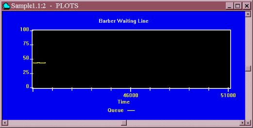
Figure 2—3. Plot Window at Completion of the Simulation

At this point we could choose to print the plot by using the Print Command from the file menu in the Plot Window. If you wish to examine the Plot in more detail, you may do this now.

Notice that the value of Q$Barber changes in vertical jumps. Such changes are happening at discrete instants. A plotted value is sampled after every Block entry in the simulation. Each time the value changes, a message is sent to the Plot Window.

You will have noticed that when the simulation completed, GPSS World wrote a report to the Report Window. The Report Window opens automatically at the end of a simulation run. Take a brief look at the Standard Report.

You can examine the report by resizing the window, or you can print the report for more detailed study later. In a later lesson, we will study the sequencing and file structure of reports in GPSS World. When you are finished with the report, close the window.

CLICK ON The X in the Upper Right-Report Window

Now that the simulation has ended, let us explore some results. The SHOW Command is ideal for this. Make sure that the Journal Window has the focus so that you can see the results of the Show Command.

CHOOSE Command / SHOW

and

TYPE C1

then

SELECT OK

This command causes the relative system clock value to be written in the Status Line as well as in the Journal. The value is the simulated time when our first simulation ended.

Let’s try one more. This time, after you have selected SHOW and the dialog box is open

TYPE QM$BARBER

SELECT OK

This shows the maximum content of the Queue Entity named Barber. If you would like to try your own favorite SNA at this time, please do so.

GPSS World allows you to view the simulation environment in many different ways. Each of the major GPSS Entity types has a window for viewing its dynamics as the simulation runs. In addition, there are Snapshots that can be viewed in a window or printed. Also, you can open the Expressions Window, which can contain a list of Labeled Expressions. Each Expression can be any valid PLUS expression. The most simple ones are variables or SNAs. The Windows are updated dynamically while the Snapshots show the state of a particular chain, group or Transaction at one point in simulated time.

Let’s open an Expressions Window on the Clock, the Customer Queue Length, and the Active

Transaction number.

CHOOSE Window / Simulation Window / Expressions Window

Then, Edit the Expressions Window

Next to Label

TYPE Clock

and for the Expression

TYPE AC1

Then, you can choose one or both of the View or Memorize options. Remember as in the Plot Window, View will allow you to see the expression(s) for this run only while memorize will allow you to use the expression(s) in future runs without having to type all the information again.

CLICK ON View

CLICK ON Memorize

If you have done this lesson from the beginning, you see that if you memorized the Q$Barber in the Plot Window, it is accessible here as well. See the Plot and Expressions Windows in the Reference Manual for more detail.

After the initial Expression is entered, for each additional Expression, you only have to type new values in the Label and Expressions boxes and then choose View or Memorize or both.

In the box for the Label

TYPE Act Trans

and for the Expression

TYPE XN1

then

CLICK ON View

CLICK ON Memorize

Finally, If you wish to view the Barber Queue,

CLICK ON The expression Q$Barber

in the Memorized Expressions box then

CLICK ON View

SELECT OK

We now will be able to view the Clock, Active Transaction Number, and size of the Barber Queue while the simulation runs.

Figure 2—4. The Expressions Window

While the simulation is running, let’s also open the Facilities Window to look at the GPSS Facility Entity which represents the barber. Don’t forget, you can interrupt a simulation by

pressing b + a + H or o.

First, close the Plot Window since we no longer wish to watch it.

DOUBLE-CLICK ON The Block Icon in the Upper Left-Plot Window

CHOOSE Window / Simulation Window / Facilities Window

Position the two windows so that you can see both as the simulation runs.

Figure 2—5. The Expressions Window and the Facilities Window

Now start a simulation. We will suppress the Standard Report this time by using NP (for "No Printout") in operand B of the START statement.

CHOOSE Command / START

In the dialog box, replace the 1.

TYPE 100000,NP

SELECT OK

Now, you can watch the vital statistics of the barber change according to conditions in the simulation, as well as watch the values of specific interest to you in the Expressions Window. The details of the Facilities Window are described in Chapter 5 of the GPSS World Reference Manual.

Watch the statistics as the simulation runs. We have one very busy barber.

It’s easy to open any of the simulation windows in this manner. However, in our simple barber shop simulation we have not defined enough entity types to make use of the other windows.

Let’s do one more thing before we end the simulation. First, let's halt the simulation.

PRESS o

or

CLICK ON The Halt icon in the Facilities Window Debug Toolbar

Then, close the Expression and Facilities Windows. Next open the Blocks Window.

CHOOSE Window/ Simulation Window / Blocks Window

We’ll use this window to put a Stop Condition on a Block, and trap a Transaction. We will choose the DEPART Block to stop a Transaction.

Halting interrupts the simulation and clears out any Queued Commands that have not yet begun. In our current simulation, there were no additional Queued Commands to be deleted. If there has been, they would be gone forever. The interrupted state of the simulation is easily restarted by a CONTINUE Command, which is itself a Queued Command.

Now let’s set a Stop Condition. In the Blocks Window,

CLICK ON The DEPART Block Icon

CLICK ON The Place Icon in the Debug Toolbar at the Top of the Window

Figure 2—6. The Blocks Window with a Selected DEPART Block

Now, restart the simulation.

PRESS m

or

CLICK ON The Continue Icon in the Debug Toolbar at the Top of the Window

The simulation will stop when the next Transaction tries to enter the DEPART Block. At this point, in the Model Window menu

CLICK ON Anywhere on the Journal / Simulation Window

to give it the focus.. Move the window to a convenient place for viewing along with the Blocks Window. You may have to resize the windows to do this.

Now, let’s send a Block Statement to the simulation.

CHOOSE Command / Custom

in the dialog box and

TYPE Trace

This will cause the Trace Indicator to be set in the Active Transaction. From now on, each Block

entry by this Transaction will cause a trace message to be sent to the Journal Window.

We have just used Manual Simulation Mode to pass a Transaction through a Block that does not become a permanent part of the model. Look at the Journal Window to see the first Trace message. Now we must remove the Stop Condition or every Transaction will be detained before entering the DEPART Block. Make the Blocks Window the active window.

CLICK ON Anyplace on the Blocks Window

CLICK ON The DEPART Block in the Blocks Window

CLICK ON The Remove Icon in the Debug Toolbar at the Top of the Window

to remove the Stop Condition on the DEPART Block. You could remove one or multiple STOP conditions by selecting Window / Simulation / Snapshot / User Stops. Try it if you like to see the User Stops Window.

Then CONTINUE the simulation.

CLICK ON The Continue Icon in the Debug Toolbar at the Top of the Window

or

PRESS m

or

PRESS b + a+ C

This will allow us to view trace messages as they are produced by the simulation.

You will see the rest of the trace messages for this Transaction until it enters the TERMINATE Block. Notice that there were no trace messages generated as other Transactions moved while the traced Transaction was delayed in the ADVANCE Block.

Figure 2—7. Trace Messages in the Journal Window

If you wish to have trace messages for all the Transactions in the model, you should insert a TRACE Block in the model. However, this is rarely necessary. It is usually much better to selectively trace Transactions in portions of the model where their behavior is not as you expected.

Don’t forget you can print the Journal at any time by making the Journal Window the active window and choosing PRINT from the FILE menu in that window.

Let’s interrupt the simulation.

CLICK ON The Halt Icon in the Debug Toolbar at the Top of the Window