

CHOOSE Command / START
and
SELECT OK
Your plot should look like this.
Figure 16—2. Sine Wave Plot.
As you can see, the familiar sine wave unfolds for both variables. When the simulation completes, examine the Standard Report. Compare the x_ variable with the Savevalue x_exact, which is calculated from the analytic solution. Do the values agree?
When you have the solution to the differential equations, consider yourself lucky and use it everywhere you can. Most real world systems of equations are much too unwieldy for that. Usually, you will be forced to play out the integration numerically, using one or more INTEGRATE Commands, which takes a lot more computer time.
Now, close all open windows.
We.., that's all for now. In the next lesson, we will learn about GPSS World's built-in Programming language called PLUS.
Lesson 17 - PLUS
This lesson considers PLUS, the Programming Language Under Simulation. See the "PLUS Primer" at the end of this lesson for practical examples of the use of PLUS.
As we have learned, Model Statements are the building blocks of Models, and they can be sent interactively to an existing simulation.
However, the only PLUS Statements that are Model Statements are the
PROCEDURE and EXPERIMENT Statements. All other PLUS Statements can exist only within the body of a Procedure. PLUS Expressions are a little different. They can exist within PLUS Statements, or, when parenthesized, within the operands of GPSS Statements.
There are only a few different PLUS Statement types. They are: EXPERIMENT — Define a PLUS Experiment.
PROCEDURE — Define a PLUS Procedure.
TEMPORARY — Define and restrict the scope of a User Variable. TEMPORARY MATRIX — Define and restrict the scope of a Matrix Entity. BEGIN / END — Compound Statement. Create a block of PLUS Statements. Assignment — Set the value of a Named Value or Matrix element. Procedure Call — Invoke a Library Procedure.
IF / THEN — Test an expression and act on a "TRUE" result. IF / THEN / ELSE — Test an expression and act on the result. WHILE / DO — Perform action repetitively.
GOTO — Jump to a new location within the Procedure.
RETURN — Finish the processing and, optionally, give a result to the caller.
Please turn now to Chapter 8 in the GPSS World Reference Manual, and read about the PLUS Language.
Welcome back. Did you notice that a PROCEDURE Statement has a slot for only one statement? Usually, you will use a Compound Statement there, and it will enclose a Statement List. However, any single valid PLUS Statement goes there just as well.
In this lesson we will not use all the PLUS Statements. Here we will demonstrate the definition and interactive redefinition of Procedures, and some tips on debugging PLUS Procedures interactively.
Let’s begin by defining a Procedure that can set the value of a User Variable.
CHOOSE File / New
CHOOSE Model
Then
SELECT OK
TYPE PROCEDURE SetPop(level) Foxes = level ;
Although most Procedures are more complex, this is all that is needed to define one. It doesn’t even declare a return value, so a return value of 0 would be used by default. Return values are useful when a PLUS Procedure passes information to a calling Procedure. We don’t use it in this simple example.
Now save the model.
CHOOSE File / Save As
Then
TYPE Fox
for the name of the model and
SELECT Save
CHOOSE Command / Create Simulation
We have included the Procedure SetPop as part of the Model and then created the Simulation. Any invocations of SetPop interactively or within the simulation will now use this definition.
CHOOSE Command / SHOW
and in the dialog box
TYPE SetPop(100)
and
SELECT OK
Notice that the return value from the SetPop Procedure was 0. Let’s look at the population level.
CHOOSE Command / SHOW
and in the dialog box
TYPE Foxes
and
SELECT OK
See? The User Variable Foxes was updated when we did the first SHOW. Now lets redefine the SetPop Procedure interactively.
CHOOSE Command / Custom
TYPE PROCEDURE SetPop(level)
Foxes = level # 10 ;
and
SELECT OK
Now, when the SetPop Procedure is invoked, the population will be set to ten times the argument. Again
CHOOSE Command / SHOW
and in the dialog box
TYPE SetPop(100)
and
SELECT OK
Notice that the return value from the SetPop Procedure was 0 again. We could have inserted a RETURN Statement into SetPop. In fact, SetPop could be
nothing more than a single RETURN Statement.
Let’s look at the population level.
CHOOSE Command / SHOW
and in the dialog box
TYPE Foxes
and
SELECT OK
As you can see, although the simulation had already been sent to the Simulation Object, we were able to redefine the Procedure interactively. This is very useful when you need to debug your own PLUS Procedures, as we will discover next.
Debugging PLUS Procedures
Let’s define a Procedure with an error in it.
CHOOSE File / New and since Model is already highlighted
SELECT OK
Enter the following PLUS Procedure.
TYPE PROCEDURE RabbitRate() BEGIN
TEMPORARY BirthRate, DeathRate, TotRate; BirthRate = 100;
DeathRate = 80 ;
RETURN TotRate; END;
Don’t forget the final semicolon. Now, save the model.
CHOOSE File / Save As
Then for the name of the file
TYPE Rates
SELECT Save
Next create the simulation
CHOOSE Command / Create Simulation
So far, so good. If you inadvertently made typing errors, use Search / Next Error in the Model Window to find and correct them. Now invoke the Procedure.
CHOOSE Command / SHOW
and in the dialog box
TYPE RabbitRate()
and
SELECT OK
We got an error message. Take a close look at each line in the message. It tells us the line number where the error occurred. Let’s put the cursor at that point. Make sure that the Model Window has the focus.
CHOOSE Search / Go To Line
TYPE 5
and
SELECT OK
Apparently, this line is trying to use a value from a Temporary User Variable that was never initialized. As we can see this is true for the TotRate Variable. We forgot to initialize it. Just above the line in error,
TYPE TotRate = BirthRate - DeathRate ;
This time we are NOT going to Retranslate the Model. We are going to redefine the Procedure and still maintain the existing simulation environment. We do this by using an Interactive INCLUDE Command. This may seem cumbersome, but it is meant to show you the power of the INCLUDE Command.
First, copy the text in the Model Window to the Window Clipboard. Next, we will create a text file.
CHOOSE File / New
SELECT Text File
SELECT OK
and then paste the Clipboard contents into the new Text File and save the file.
CHOOSE File / Save As
TYPE RateDef
for the file name and
SELECT Save
This creates a TEXT file that can be used as the Include File. All Include Files must be text files. Now, let’s redefine SetPop( ) in the existing simulation. That means using INCLUDE, not Retranslate.
CHOOSE Command / Custom
and in the dialog box
TYPE INCLUDE "RateDef.txt"
and
SELECT OK
So far, so good. Notice that we did not Retranslate. Now invoke the Procedure.
CHOOSE Command / SHOW
and in the dialog box
TYPE RabbitRate()
There. That fixed the problem. It was easy to redefine the Procedure interactively. Although it was not so important here, in a big simulation you may not want to disturb the simulation. That’s when interactive redefinition really pays off. In such cases, you may want to load an INCLUDE Command into a function key, and use it to read in a small file containing nothing but the test definition of the Procedure. The main thing to remember is that you must save changes before you use INCLUDE. A DO Command is also useful for debugging Plus Procedures. See Chapter 8 in the Reference Manual.
You may find it convenient to make minor modifications to the PLUS Procedure when you are testing it. First, you may want to "comment out" TEMPORARY Statements, as long as none of the Temporary User Variable or Matrix Names clash with global entities. If there is a conflict, global variables could be altered. It is best to keep the Temporary names unique. Simply place /* at the beginning of each TEMPORARY or TEMPORARY MATRIX Statement, and */ after it. This will cause your intermediate results to be available after the Procedure ends. Second, you can add additional Assignment Statements and RETURN Statements to stop the Procedure wherever you like.
Then to test the results, all you have to do is redefine the Procedure and invoke it. Each action could be done with a single stroke of a Function Key. The highly interactive GPSS World environment makes Procedure redefinition an effective debugging technique.
A few other items of interest include the fact that PLUS Procedures can call other PLUS Procedures and can be accessed from any block operand in your model as well as from the PLUS block.
Hopefully, reviewing the example models in this lesson and the examples in the Plus Primer that follows will help you to understand some of the potential of PLUS. Also, the sample model PREDATOR.GPS in Chapter 2 of this manual uses a PLUS Procedure. There’s a World of power waiting for you.
Lesson 18 - Debugging Your
Models
GPSS World’s interactivity makes debugging and the testing of design alternatives much easier than in older versions of GPSS. In the last lesson we saw how much easier it is to debug PLUS Procedures in an interactive environment. In this lesson, we’ll try a few simple debugging techniques that can be very useful when you apply them to complex models.
The model is shown below.
;GPSS World Sample File - BARBER.GPS.
***********************************************************************
* *
* Barber Shop Simulation *
* *
***********************************************************************
Waittime QTABLE Barber,0,2,15 ;Histogram of Waiting times GENERATE 3.34,1.7 ;Create next customer
TEST LE Q$Barber,1,Finis ;Wait if line 1 or less
;else leave shop
SAVEVALUE Custnum+,1 ;Total customers who stay
ASSIGN Custnum,X$Custnum ;Assign number to customer
QUEUE Barber ;Begin queue time
SEIZE Barber ;Own or wait for barber
DEPART Barber ;End queue time
ADVANCE 6.66,1.7 ;Haircut takes a few minutes
RELEASE Barber ;Haircut done. Give up the barber
Finis TERMINATE 1 ;Customer leaves
CHOOSE File / Open
SELECT BARBER
and
SELECT Open
Before we go any further, let’s put some SHOW commands into Function Keys. Open the Model Settings Notebook
CHOOSE Edit / Settings and select the Function Keys page.
Next to s and t type the following two SHOW Commands. Place the mouse pointer in each box and click once before typing.
TYPE SHOW P$Custnum
and
TYPE SHOW X$Custnum
SELECT OK
You have now loaded SHOW commands into two function keys. While debugging a simulation you can interactively examine many values at a touch of a single key. We’ll use them later.
Now create the simulation.
CHOOSE Command / Create Simulation
Let’s also open the Blocks Window. In the Main Menu
CHOOSE Window / Simulation Window / Blocks Window
Now, let’s put a Stop Condition on Transaction 5.
CHOOSE Command / Custom
and in the dialog box
TYPE Stop 5
SELECT OK
You should also arrange the windows so you can see both the Blocks Window and the Journal Window.

Your screen should look something like this.
Figure 18—1. The Blocks, and Journal Windows in BARBER.GPS.
In the Main Menu
CHOOSE Command / START
and in the dialog box replace the 1
TYPE 100
and
SELECT OK
Now you see a message indicating that Transaction 5 has stopped on its first attempted Block entry in the simulation. In this case it happens to be the first GENERATE Block.

Figure 18—2. Message after Stop is executed in the Journal Window.
Now, we’ll step through the simulation using the function key that is loaded in the Model Settings Notebook with STEP 1. If you want to check the list of preassigned function key settings, go to the Function Keys Page of the Model Settings Notebook.
Now that we have control of the active Transaction, let’s first take off the Stop Condition.
CHOOSE Window / Simulation Snapshot / User Stops
CLICK ON The "5"
CLICK ON The Remove Button
SELECT OK
PRESS p
You could also execute this command by pressing b+a + S or choosing Command / STEP in the Main Menu.
Transaction 5 will enter the GENERATE Block. You’ll be able to see this in the trace messages in the Journal Window. Now STEP one more time to cause the Transaction to enter the TEST Block.
PRESS p
When this Transaction enters the TEST Block, it will find that the queue for the barber is greater than 1. This customer will then choose not to wait and will leave the shop. You will see it has been scheduled for the TERMINATE Block.
Now, before going on, let’s examine some other values related to the simulation.
CHOOSE Command / SHOW
and in the dialog box
TYPE Q$Barber
and
SELECT OK
and see that the size of the queue (2) is returned to the Status Line in the Main
Window, but can also be seen in the Journal Window. Now, let’s use the SHOW Commands that we loaded into the function keys.
PRESS t
The value 4 will be returned in the Status Line. This tells us the number of customers who have stayed at the shop. Remember, you can also use the Expressions Window to watch a whole series of values as you step through a simulation. The Expressions Window was discussed in detail in the Lesson 11. Now let’s continue to Step through the simulation.
PRESS p
to move Transaction 5 through the TERMINATE Block. Now let’s look at the number of customers that have stayed in the shop
PRESS t
The value returned will be 4. Transaction 5 did not wait and was not added to our counter.
We’ll use the preloaded function key for CONTINUE to do this
PRESS m
If the Blocks Window is open, the simulation will run more slowly than with all the windows closed. Close the Blocks Window now, but minimize the Journal Window for later use.
CLICK ON The X-Upper Right of the Blocks Window
then
CLICK ON The leftmost of the three buttons-Upper Right of the Journal Window
The simulation will quickly run to completion and a report will be written. Let’s also take a quick look at one of the other windows, the Table Window.
CHOOSE Window / Simulation Window / Table Window
and in the drop-down box, you’ll see Waittime, since this is the only Table in the model.
SELECT OK
In this particular histogram you can see the wait times experienced in the queue for the barber. Mean waiting time was 10.709 minutes with a standard deviation of 2.702 minutes. The Table Window is dynamic, and is updated as the state of the simulation changes.
Figure 18—3. The Waittime Table
Before we go on, let’s restore the Journal Window. On the Desktop CLICK ON The Minimized Icon in the lower left of the screen
Now we can watch Journal messages as we work a little more with the use of Stops.
CHOOSE Window / Simulation Window / Blocks Window and open the Blocks Window to a comfortable viewing size.
Now, in the Blocks Window select the RELEASE Block (Block number 9) in the model. You can do this by moving the mouse pointer over the Block labeled REL and clicking mouse button 1.
CLICK ON The Release Block in the Blocks Window then
CLICK ON The Place Icon in the Debug Toolbar
A Stop Condition has now been put on Block 9. You can do this through the Command menu in the Main Window, as well using a Custom Command, but using the Debug Toolbar is easier. Now start the simulation.
CHOOSE Command / START
and in the dialog box replace the 1
TYPE 100
and
SELECT OK
The simulation will now stop when the first Transaction is ready to enter the RELEASE Block.
As you can imagine, these techniques will become even more valuable as your model becomes more complex.
The change will be implemented immediately. First Now let’s alter the structure
of the model without leaving the Session.
PRESS s
Remember, we loaded a SHOW Command for the customer number Parameter
into s early in the lesson. The value returned in the Status line of the Main Window is 54 for the Customer Number.
Let’s remove the STOP on the RELEASE Block.
CHOOSE Window / Simulation Snapshot / User Stops
CLICK ON The "9"
CLICK ON The Remove Button
SELECT OK
Now let’s assume you have decided you no longer want each Transaction to carry the customer number in a Parameter. We’ll eliminate the ASSIGN Block. In the Model Window, position the mouse at the beginning of the ASSIGN Block line.
CLICK and DRAG The Cursor to the End of the Line
and
PRESS c
Now in a flash you can retranslate the model and start it running again.
CHOOSE Command / Retranslate
and then
CHOOSE Command / START
and in the dialog box replace the 1
TYPE 11111
and
SELECT OK
Let the simulation run for a second or two and
PRESS o
to halt the simulation and then
PRESS s
Chances are you got an error message saying that the Parameter doesn’t exist since it is no longer being assigned to new Transactions. Let’s take a look at a way we can make interactive changes in a simulation without having to retranslate the model. We’ll read in a new model to examine this option.
The model below deserves a little study before you see how GPSS World allows interactive changes to your simulation while you are in the development and test phases of a project. Take a minute to look at the model shown below.
; GPSS World Sample File - SAMPLE7.GPS
**********************************************************************
**
*Automobile Arrival Simulation *
**
*For simplicity, this model only deals with one-way traffic *
*in North-South and East-West directions. *
**********************************************************************
GENERATE 20,10 ;Create next automobile. QUEUE Eastwest
TEST E X$EWlight,F$Intersection ;Block until green, and
*the intersection is * * free
SEIZE Intersection
DEPART Eastwest ;End queue time. ADVANCE 10 ;Cross the intersection. RELEASE Intersection
TERMINATE 1 ;Auto leaves intersection.
*
GENERATE 30,10 ;Create next automobile. QUEUE Northsouth
TEST E X$NSlight,F$Intersection ;Block until green and
*the intersection is free SEIZE Intersection
DEPART Northsouth ;End queue time. ADVANCE 10 ;Cross the intersection. RELEASE Intersection
TERMINATE 1 ;Auto leaves intersection.
**********************************************************************
**
*Traffic Light Simulation *
**
**********************************************************************
GENERATE ,,,1
Begin1 SAVEVALUE NSlight,Red ;North-South light turns red SAVEVALUE EWlight,Green ;East-West light turns green ADVANCE Greentime ;Light is green
SAVEVALUE NSlight,Green ;North-South light turns green SAVEVALUE EWlight,Red ;East-West light turns red ADVANCE Redtime ;Light is red
TRANSFER ,Begin1 Greentime EQU 200
*When the light is Green (value 0) and the intersection is not busy
*(the State Variable(SNA) F$Intersection evaluates as 0), a car may
*pass into the intersection. These conditions are tested at the TEST
*Block. When the light is red (value 100) or the intersection is busy
*(SNA F$Intersection returns the value 1), the condition at the TEST
*Block will not be met and the car will not proceed.
Green EQU 0
Red EQU 100 Redtime EQU 300
*
*Do START 4000 EW Congestion builds. Try Greentime EQU 1000. Fine
*but NS congestion builds. Greentime EQU 400 works for both.
This model is of an intersection of two one-way streets. By changing the length of the green light, you can experiment with the effects on the traffic flow. We will open the Plot Window with two variables, one for North-South traffic and one for East-West traffic.
First, Open the model
CHOOSE File / Open
and
SELECT SAMPLE7
and
SELECT Open
Then create the simulation and open the Plot Window.
CHOOSE Command / Create Simulation
and
CHOOSE Window / Simulation Window / Plot Window
When the Edit Plot Window appears, enter the values you see below. Remember to position the mouse pointer at the start of each line and click once
before you start to type or use the v key to go from box to box in a forward direction. Don’t try to use e to go from box to box.

Figure 18—4. The Edit Plot Window.
The label field contains the label used in the legend at the bottom of the plot Next, the Expression box indicates the variable to be plotted. Finally, in the Title field we’ll choose a name that will describe both items that we want to plot, namely the Queues of cars in both directions. The Y-axis values have defaults of 0 and 100. We’ll change only the Max value to 150.
Finally, the time range for each view of the plot must be added. Our time range is 8000. You will want to make this time duration long enough so that it does not flash by as the simulation runs, but not so long that your plot is jammed together. You may have to experiment once or twice to get the correct value. The Plot Window will page horizontally when it reaches the end of the window. You should also be aware that by default only 10,000 plot points are saved for each expression. You can change this setting in the Model Settings Notebook. If you refresh or resize your window or do anything that causes the window to refresh automatically, such as dragging another window over the top of the Plot Window, only the remembered points can be redrawn. Of course, the more points you save, the more memory you will use for this purpose. Since GPSS World makes huge amounts of memory available to you, this is not usually a problem.
To add these values to the plot
CLICK ON The Plot button
and ifyou want to save the information with this simulation
CLICK ON The Memorize button
Now, you need to add the second variable that we want to plot. Enter only the new Expression and Label. For the Label replace the existing information.
TYPE North South Traffic
and for the Expression, replace the existing information
TYPE Q$NorthSouth
CLICK ON The Plot button
and ifyou want to save the information with this simulation
CLICK ON The Memorize button
SELECT OK
Position and size the window for easy viewing and then start the simulation running.
CHOOSE Command / START
and in the dialog box and replace the 1.
TYPE 4000
and
SELECT OK
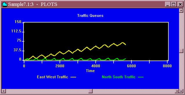
Your Plot Window should look something like this. Of course, it will depend where in simulated time you are.
Figure 18—5. Intersection Congestion when Greentime equals 200.
Notice that East-West congestion is building. Interrupt the simulation with
PRESS o
Open up a Custom Command dialog box
CHOOSE Command / Custom
and
TYPE Greentime EQU 1000
SELECT OK
then
PRESS m
This will cause the CONTINUE command to be executed. Now notice that North-South congestion builds. Interrupt the simulation again
PRESS o
Open up a Custom Command dialog box
CHOOSE Command / Custom
and
TYPE Greentime EQU 400
SELECT OK
then
PRESS m
Now the traffic is flowing reasonably in both directions. Let the simulation run to completion or you can halt it when you are done watching the Plot.
PRESS o
if you prefer.
Close all Windows related to the Traffic Model.
CLICK ON The X-Upper Right of each Window
GPSS World can also call in Command Files consisting of INITIAL statements or other Commands. You can do this either by interactively typing an INCLUDE Command in a Custom Command dialog box or by placing this statement in a Model File.
Read in the Barbershop model.
CHOOSE File / Open
and in the dialog box
SELECT BARBER
then
SELECT Open
Create the simulation
CHOOSE Command / Create Simulation
The following is an example of the command to call in an ASCII file containing Initial Statements as described above. The first command shows how it would be done interactively, the second as part of your program.
CHOOSE Command / Custom
and in the dialog box
TYPE INCLUDE "INIT.TXT"
SELECT OK
Remember, if you have altered the location of the sample files, then, you must assert the file path in this INCLUDE Command.
The contents of this file are: INITIAL X$One,45
INITIAL X$Two,765
Now show the values of these Savevalues. The SAVEVALUE entities are created as they are given their initial values.
CHOOSE Command / SHOW
and in the dialog box
TYPE X$One
SELECT OK
You should see the value 45 in the Status Line of the Main Window and in the Journal Window. Repeat this process to see the second SAVEVALUE.
CHOOSE Command / SHOW
and in the dialog box
TYPE X$Two
SELECT OK
and check the value in the Status Line.
Add the following line as the last line of the model that you currently see in the Model Window
INCLUDE "INIT.TXT"
Now let’s retranslate this model.
CHOOSE Command / Retranslate
When the model is retranslated, it will automatically read the external file and create and initial the Savevalues. Show the Savevalues as we did above, if you wish.
INCLUDE Files can also be used as we did in the ANOVA Lesson. They make it easy to manage multiple runs of a simulation. Also, unless suppressed, a report will be produced for each completed simulation run. See the GPSS World Reference Manual and Lesson 14 of this manual for more information on report options.
In this lesson, you have used some of the interactive capabilities of GPSS