Part 6. Interpolation and Extrapolation of Functions

TABLE 6.1 Comparison of the characteristics of alternative methods

Method	Error Associated with Data	Number of Points Matched Exactly	Programming Effort	Comments
Newton's Divided Difference Polynomial	Small	n + 1	Easy	Usually preferred for exploratory analyses
Lagrange Polynomials	Small	n + 1	Easy	Usually preferred when order is known
Cubic Spline	Small	Piecewise fit of data points	Moderate	First and second derivatives are equal at knots

TABLE 6.2 Summary of important information

Method	Formulation	Error
Newton (Gregory-Newton) Interpolating Polynomial
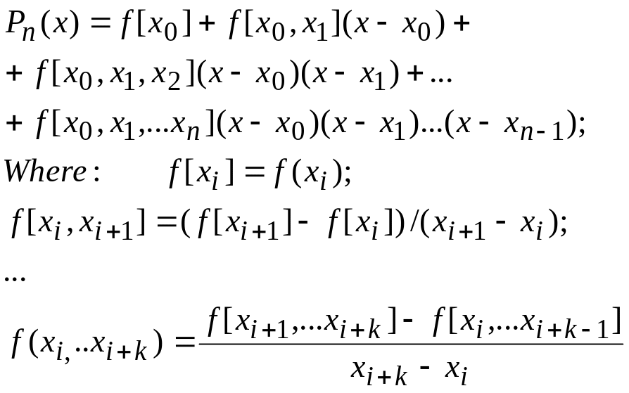
Newton's Divided Difference Interpolating Polynomial
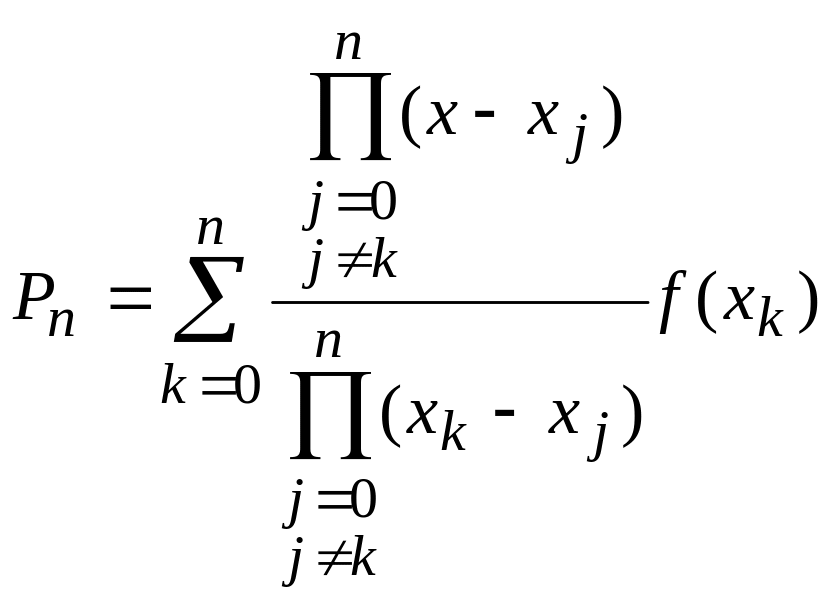
Lagrange Interpolating Polynomial
Spline Interpolation	A linear spline: , (i = 1, n). A quadratic spline: is fit to interval between knots. The first derivatives at the interior knots must be equal. A cubic spline: is fit to interval between knots. First and second derivatives are equal at each knot.

Example 1

Given the data:

x	1	2	3	4	5
f(x)	0	5	22	57	116

1. Calculate f(2.5) using the Lagrange polynomial of order 4.

2. Employ inverse interpolation using Newton's divided difference interpolating polynomial to determine the value of x that corresponds to y = f(x) = 20.

Solution. a) To find an approximate value for f(2.5), we compute P₄(2.5).

b) In this case we use the Newton polynomial reversing the variables:

Construct a table for computing the divided differences.

y	f[y]	f[.,.]	f[.,.,.]	f[.,.,.,.]	f[.,.,.,.,.]
0	1
		0.2
5	2		-6.417·10-3
		0.05882		1.024·10-4
22	3		-5.817·10-4		-8.472·10-7
		0.02857		4.127·10-6
57	4		-1.236·10-4
		0.01695
116	5

Hence ,

Example 2

Fit the data in the table below with a) first-order splines, b) quadratic splines, c) use the results to estimate the value at x = 3.3, d) compute percent relative errors for the numerical results.

x	0	1	2	3	4	5
f(x)	0	0.5	0.8	0.9	0.941176	0.961538

Note that the values in the table were generated with the function .

Solution.

a) The slopes for all intervals can be computed (see Table 6.2), and the resulting first-order splines are:

b) Now fit quadratic splines to the same data using formulas:

;

Select , then:

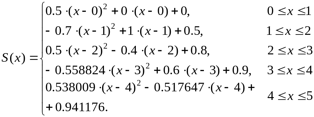
Hence,

3. The correct value of the function at x = 3.3 is f(x) = 0.915896.

4. The result of first-order splines at x = 3.3 is f(x) = 0.93. The percent relative error is ε_t = 1.5%. The result of quadratic splines at x = 3.3 is f(x) = 1.029706. The percent relative error is ε_t = 12.4%.

Problems

1. Given the data:

x	1	2	2.5	3	4	5
f(x)	1	5	7	8	2	1

Calculate f(4.4) using a) Newton (Gregory-Newton) interpolating polynomial, b) Newton's divided difference interpolating polynomial.

2. Employ inverse interpolating to determine the value of x that corresponds to f(x) =1.0 for the following tabulated data:

x	1.0	1.2	1.4	1.7	2.0
f(x)	0.5652	0.7147	0.8861	1.1964	1.5906

a) Use the linear splines; b) Use the Lagrange polynomial.

3. Develop cubic splines for the following tabulated data:

x	1	2	3	5	6
f(x)	4.75	4	5.25	19.75	36

a) Calculate f(2.5) and f(4.0); b) Verify that S₃(5) = S₄(5).