Practise Part 1. Error and Accuracy of Calculations

The errors associated with both calculations and measurements can be characterized with regard to their accuracy and precision:

• Accuracy refers to how closely a computed or measured value agrees with the true value.

• Precision refers to how closely individual computed or measured values agree with each other.

The numerical error is equal to the discrepancy between the truth and the approximation, as in

E_t = true value - approximation.

The true percent relative error is determined according to

.

The percent relative error is determined according to

.

We can be assured that the result is correct to at least n significant figures

.

For such cases, the computation is repeated until

.

Problems

1. The infinite series 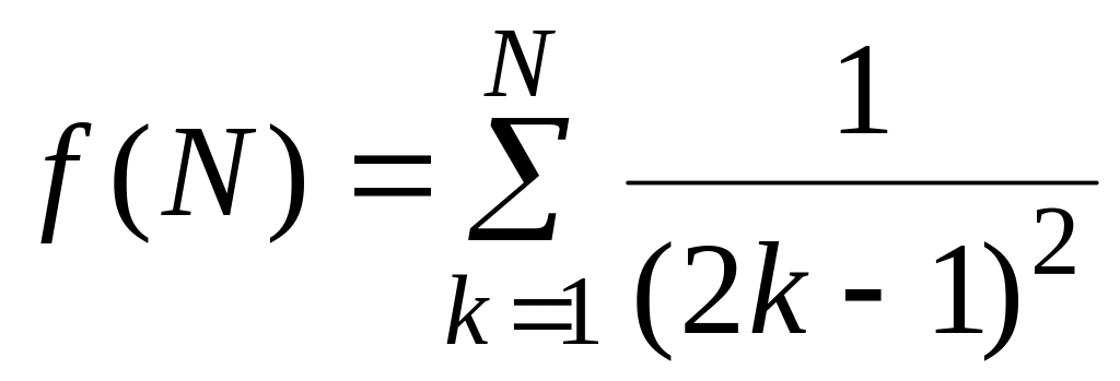converges on a value of as N approaches infinity. Write a program to compute 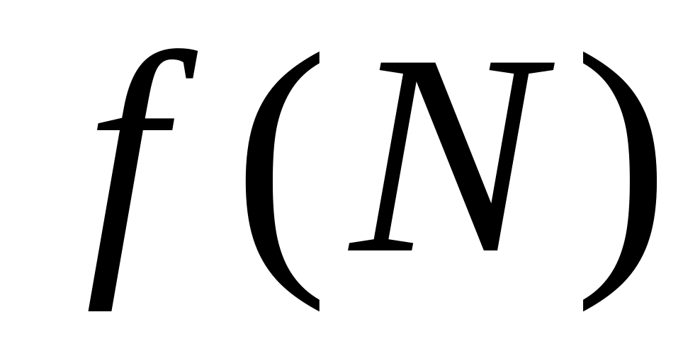for N = 10 000 by computing the sum from k = 1 to 10 000. Then repeat the computation but in reverse order - that is, from k = 10 000 to 1 using increments of -1. Explain the results.

2. The Maclaurin series expansion for cos x is

Starting with the simplest version, cos x = 1, add terms one at a time to estimate . Add terms until the absolute value of the approximate error estimate falls below a prespecified criterion conforming to four significant figures. Use your pocket (PC) calculator to determine the true value.

3. Perform the same computation as in Prob. 2, but use the Maclaurin series expansion for sin x,

to estimate .

Part 2. Numerical Integration

TABLE 2.1 Important integration formulas

Method	Formula	Error
Left Sum Approximation		O(h)
Right Sum Approximation		O(h)
Midpoint Approximation		O(h2)
Trapezoidal Approximation		O(h2)
Simpson’s (1/3) Approximation		O(h4)
Simple Monte Carlo Approximation		

^* ; ^** .

Example 1

Suppose we want to evaluate the integral . The definite integral is the area under the curve , above the x-axis and between the lines x = 0 and x = 10. The actual value can be easily obtained as follows:

.

Solution. n = 4 (h = 2.5)

a) Use it in conjunction with Left sum approximation to integrate the same function for four subintervals:

.

The numerical error and the true percent relative error are:

.

2. Using Right sum approximation:

.

.

2. Using Trapezoidal Rule (four subintervals):

.

.

2. Using Simpson's 1/3 Rule (four subintervals):

.

.

Example 2

Suppose we want to evaluate the following double integral:

.

For the numerical evaluations use both the trapezoidal and Simpson's 1/3 rules. For both cases, use the multiple-application version, with n = 4. Compute percent relative errors for the numerical results.

Solution.

a) Analytically the actual value can be easily obtained as follows:

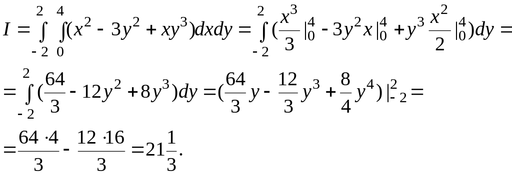
b) Numerical integration with n = 4: (h_x = 1.0; h_y = 2.0)

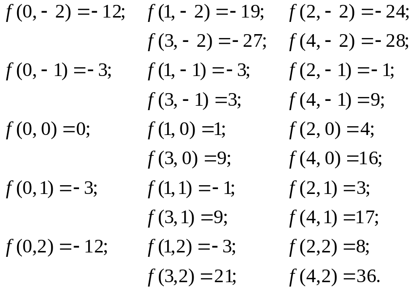
3. Use it in conjunction with Trapezoidal Rule to integrate the same function for four subintervals:

.

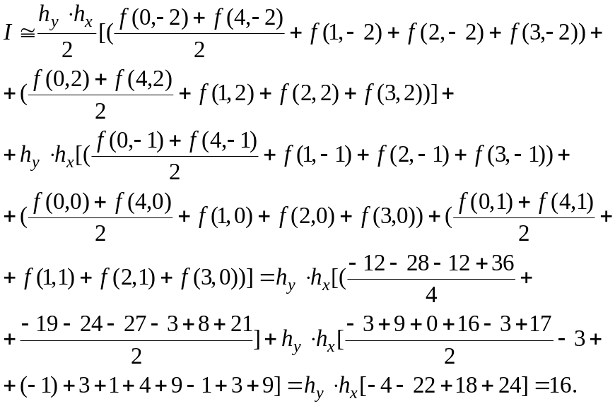
d) Using Simpson's 1/3 Rule:

.

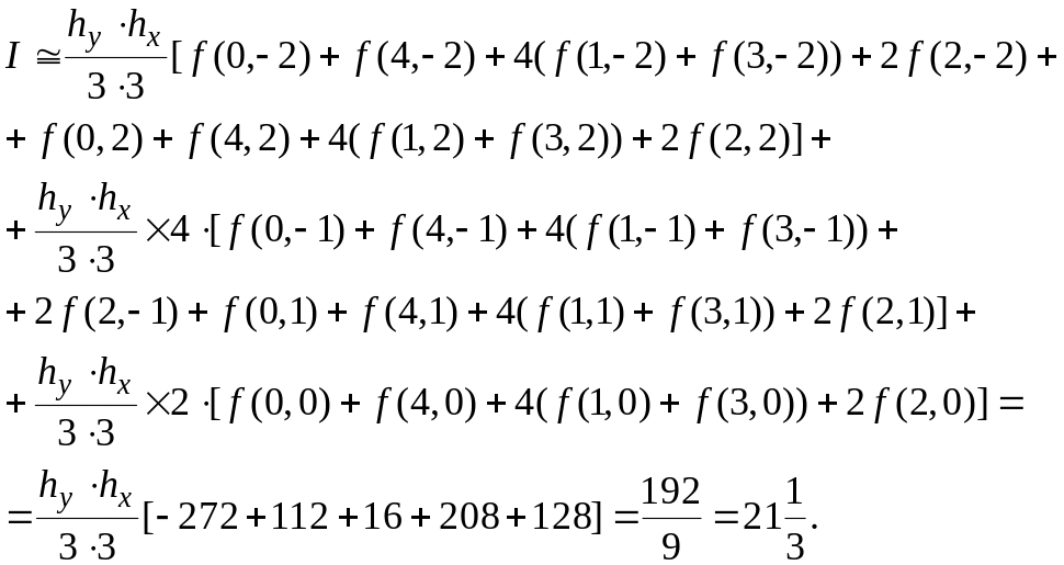
Note:

• Trapezoidal rule gives the exact value of the integral for linear polynomials;

• The Simpson's rule gives the exact value of the integral for polynomials of degree three or less;

• An even number subintervals must be utilized to the Simpson's rule;

• As the number of subintervals increases, the approximations get better.

Problems

1. Integrate the following function both analytically and numerically.

.

For the numerical evaluations use: (a) left sum approximation, (b) right sum approximation, and (c) midpoint approximation. For all cases use version with n = 4. Compute percent relative errors for the numerical results.

2. Integrate the following function:

.

Note that the true value is I = 0.602297. Use both the trapezoidal and Simpson's 1/3 rules to numerically integrate the function with n = 4.

3. Evaluate the triple integral

(a) analytically, and (b) using Simpson's 1/3 rule with n = 4. For (b) compute the percent relative error ( ).

4. Integrate the following function both analytically and numerically.

.

For the numerical evaluations use: (a) midpoint approximation, (b) Monte Carlo integration.

A random sample ( ) of size 20 is given below:

i		i		i		i
1	0.0105	6	0.2171	11	0.2747	16	0,4150
2	0.0039	7	0.5369	12	0.4442	17	0.1651
3	0.3351	8	0.1957	13	0.1089	18	0.8154
4	0.0332	9	0.7003	14	0.6982	19	0.6855
5	0.3557	10	0.9498	15	0.5643	20	0.7643

For all cases use version with n = 10. Compute percent relative errors for the numerical results. Discuss your results.

5. The function

can be used to generate the following table of unequally spaced data:

x	0.0	0.12	0.22	0.32	0.36	0.40	0.44	0.54
f(x)	0.20000	1.309729	1.305241	1.743393	2.074903	2.456000	2.842985	3.507297

Evaluate the integral from a = 0 to b = 0.54 using: (a) analytical means, (b) left sum approximation, (c) right sum approximation, and (d) the trapezoidal rule. For (b), (c) and (d), compute the percent relative error ( ).