DC14Sample

Добавил:

Upload Опубликованный материал нарушает ваши авторские права? Сообщите нам.

Вуз:

Национальный авиационный университет

Предмет:

[НЕСОРТИРОВАННОЕ]

Файл:

So, immediately, one has

uncorrected

.pdf

Скачиваний:

Добавлен:

19.02.2016

Размер:

1.06 Mб

Скачать

☆

<<< < Предыдущая 1 2 3 45 / 65 6 > Следующая >>>

This electronic version is for personal use and may not be duplicated or distributed.

6.6. Optimal Controller Design							223
1.4						proofs
1.2				20		proofs
				20

1				10
				10
0.8
				0
0.6
0.4				−10
0.2				−20
				−20
0
0	5	10	15	0	5	10	15
	(a) output signal				(b) control signal
	Figure 6.28. Step response of the system when saturations are introduced.
uncorrected
		Figure 6.29. OCD interface.
6.6.3 A MATLAB/Simulink-Based Optimal Controller Designer and
	Its Applications
From the examples in the previous section, using numerical optimization algorithms, optimal
controller design can be made simple. In this section, we will introduce a Matlab/Simulink-
based optimal controller designer (OCD) with some application examples.
The procedures for applying the OCD program are as follows:

1.Type ocd at the MATLAB prompt; the main interface is shown in Fig. 6.29. The program can be used in optimal controller design.

From "Linear Feedback Control" by Dingyu Xue, YangQuan Chen, and Derek P. Atherton. This book is available for purchase at www.siam.org/catalog.

This electronic version is for personal use and may not be duplicated or distributed.

224		Chapter 6. PID Controller Design
2.	A Simulink model can be established and the model should contain at least two
			proofs
	elements: the undetermined variable names and the outport reﬂecting the optimum
	criterion. For instance, in the PI controller design problem, the two variables Kp and
	Ki can be assigned. The ITAE criterion can be represented in the Simulink model as
	outport 1.
3.	Fill in the Simulink model name in the Select a Simulink model edit box.
4.	Fill in the variable names to be optimized in the Specify Variables to be optimized
	edit box, with variable names separated with commas.
5.	Estimate the terminate time for the error to become zero and enter it in the Simulation
	terminate time edit box.

6. Click Create File to automatically generate a MATLAB function optfun *.m and click Clear Trash to delete the temporary objective function ﬁles.

7. Click Optimize to start, the optimization process. The optimal variables can be obtained. Sometimes, the button should be clicked again to ensure more accurate optimum solutions. The functions fminsearch(), nonlin() and fmincon()

can be called automatically for parameter optimization.
uncorrectedFigure 6.30. PID control model and response comparisons.
8. The upper and lower bounds to the variables can also be used, and initial search point
can be speciﬁed, if necessary.
Example 6.21. Consider the FOIPDT-type plant model in Example 6.15; i.e., the plant
model is given by
G(s) = s(s	1	1)4 .
	+

The Simulink model for the PID control, with ITAE descriptions, is established as shown in Figure 6.30(a), and it is saved in the ﬁle c6mopt4.mdl.

Fill in the Simulink model name in the Select a Simulink model edit box, for instance, ﬁll in c6mopt4 for this example. The variable names to be optimized, Kp,Ki,Kd should be entered in the SpecifyVariables to be optimized edit box, and enter 30 in the Simulation terminate time edit box. Then click the Create File button to automatically generate the MATLAB function to describe the objective function

	1	1					Step Response
\|u\|	s	1					Step Response
\|u\|	s			1.6
				1.6
				1.4	PD controller
Kp				1.4		↓
Kp						↓
				1.2		← PID controller
			Amplitude			← PID controller
Ki	1			1
Ki	1
s	s(s+1)(s+1)(s+1)(s+1)			0.8	← optimum controller
Step	Zero−Pole	Scope		0.6	← optimum controller
Step	Zero−Pole
Kd.s				0.4
0.01s+1				0.2
				0
				0	5	10	15	20	25	30
							Time (sec)
(a) Simulink model (ﬁle: c6mopt4.mdl)						(b) comparisons

From "Linear Feedback Control" by Dingyu Xue, YangQuan Chen, and Derek P. Atherton.

This book is available for purchase at www.siam.org/catalog.

6.6. Optimal Controller Design

This electronic version is for personal use and may not be duplicated or distributed.

225

	function y=optfun_2(x)
2	assignin(’base’,’Kp’,x(1));
3	assignin(’base’,’Ki’,x(2));
4	assignin(’base’,’Kd’,x(3));
5	[t_time,x_state,y_out]=sim(’c6mopt4.mdl’,[0,30.000000]);
6	y=y_out(end);

		proofs

where the second, third, and fourth lines in the code will assign the variables in vector x to the variables Kp, Ki, Kd in the MATLAB workspace. Simulation is then performed to calculate the objective function.

Click the Optimize button to initiate the optimization process. In the meantime, the scope window should be opened to visualize the optimization process. After optimization,

the optimum PID controller will be obtained as
Gc(s) = 0.2583 +	0.0001	0.7159s
	s	+ 0.01s	+	1

which minimizes the ITAE criterion. It can be seen that Ki = 0.0001 is very small, which
uncorrectedFigure 6.31. Simulation model of cascade PI control (ﬁle: c6model2.mdl).

can be neglected, and thus a PD controller is sufﬁcient for the system. The closed-loop step response is shown in Fig. 6.30(b). It can be seen that the control response is highly superior to the one obtained in Example 6.15.

Example 6.22. The OCD program is not restricted to simple PID controller problems. It can also be used for complicated system models such as the cascade PI control system shown in Fig. 2.11.

To solve the problem, the Simulink model shown in Fig. 6.31 can be established, and saved as c6model2.mdl. Note that four undetermined parameters Kp1, Ki1, Kp2, Ki2 should be optimized. The ITAE criterion can be deﬁned. Starting the OCD, the model name c6model2 should be entered into the Select a Simulink model edit box, and in the Specify Variables to be optimized edit box, Kp1,Ki1,Kp2,Ki2 should be ﬁlled in. Also, in the Simulation terminate time edit box, one may ﬁll in 0.6. Click the Create File to generate the MATLAB function. One may design the controllers by clicking the Optimize button, and the controllers, which minimize the ITAE criterion, can be found as Kp1 = 37.9118,

time

|u|

0.212

Abs

Kp1.s+Ki1

0.1

Kp2.s+Ki2

0.21

130

0.01s+1

0.0067s+1

0.15s+1

Step

Outer PI

Filter

Inner PI

Thyrister

Scope

Controller

0.1

0.01s+1

Current with filter

0.0044

0.01s+1

Speed with filter

From "Linear Feedback Control" by Dingyu Xue, YangQuan Chen, and Derek P. Atherton.

This book is available for purchase at www.siam.org/catalog.

This electronic version is for personal use and may not be duplicated or distributed.

226		Chapter 6. PID Controller Design
	250	proofs
	200	proofs
	200
	150
	100
	50
	0


0	0.1	0.2		0.3	0.4	0.5	0.6
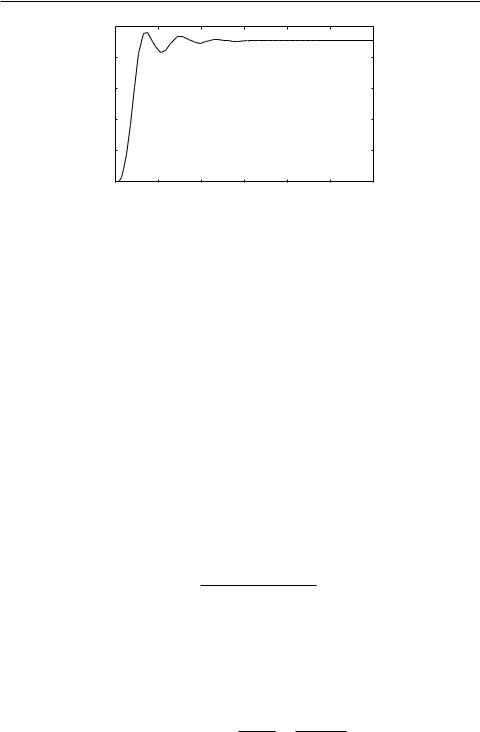
	Figure 6.32. Optimal control of the system.
Ki1 = 12.1855, Kp2 = 10.8489, and Ki2				= 0.9591, i.e., the controllers are
		12.1855						0.9591
uncorrected
Gc1 (s) = 37.9118 +			s	and	Gc2 (s) = 10.8489		+	s	.

Under these controllers, the step response of the closed-loop system can be obtained as shown in Fig. 6.32. It can be seen that the response is satisfactory.

It can be seen from the previous examples that the OCD program is quite versatile in ﬁnding the optimal controllers. However, in some applications, the OCD may not ﬁnd a solution due to the poorly posed problem or because a good initial search point has not been found. This can be a drawback in conventional optimization algorithms, but many such problems can be avoided by intelligent use based on an understanding of the system behavior.

The genetic algorithm (GA) [77] allows the optimization search from many initial points in a parallel manner. The Genetic Algorithm Optimization Toolbox (GAOT) [78] provides a series of MATLAB-based functions for solving optimization problems using genetic algorithms. This toolbox is used with the OCD program, and the facility is useful in solving problems where conventional optimization methods cannot easily ﬁnd an initial feasible search point. The GA Optimization Toolbox is the last list box in Fig. 6.29.

Example 6.23. Consider an unstable plant model

s + 2

G(s) = s4 +8s3 +4s2 −s+0.4 .

By the direct use of the OCD program, a feasible PID controller cannot be designed. However, one may still establish a Simulink model as shown in Fig. 6.33, which is the same as the previous examples.

In order to ensure that the control action is not too large, a saturation element can be appended to the controller, with the saturation width of = 5. From the OCD program, with the GAOT selection, the optimal PID controller can be designed as

Gc(s) = 47.8313 + 0.2041 + 55.3632s . s 0.01s + 1

From "Linear Feedback Control" by Dingyu Xue, YangQuan Chen, and Derek P. Atherton.

This book is available for purchase at www.siam.org/catalog.

This electronic version is for personal use and may not be duplicated or distributed.

6.7. More Topics on PID Control						227
time			1/s		1
time	\|u\|
	\|u\|				ITAE criterion
					ITAE criterion
	Ki(s)
	s
	Ki			s+2
	Kp			s+2
	Kp		s4+8s3+4s2−s+0.4
Step	Kp	Saturation	s4+8s3+4s2−s+0.4			Scope
Step	Kp	Saturation				Scope
	Kd.s		unstable plant
	0.02s+1
	approximate Kd
Figure 6.33. Simulink model for PID control (ﬁle: c6munsta.mdl).
1					proofs
0.8
0.6
0.6
0.4
0.2
0
0	2	4	6		8	10
Figure 6.34. Simulation results for an unstable plant with a PID controller.
uncorrected
The step response of the closed-loop system under the optimal controller is shown in
Fig. 6.34. It can be seen that the PID controller can still be designed, with the help of GAs,
and the transient response is satisfactory.

6.7 More Topics on PID Control

6.7.1 Integral Windup and Anti-Windup PID Controllers

A Simulink model for the study of the phenomenon of integrator windup is shown in Fig. 6.35.

The plant model is given by
10
G(s) =		,
	s4 + 10s3 + 35s2 + 50s + 24

From "Linear Feedback Control" by Dingyu Xue, YangQuan Chen, and Derek P. Atherton.

This book is available for purchase at www.siam.org/catalog.

This electronic version is for personal use and may not be duplicated or distributed.

228			Chapter 6. PID Controller Design
				3
				proofs
				Out3
				2
				Out2
	Kp	1		num(s)
	Kp			1
		Ti.s		den(s)
Step	Gain			Out1
		Transfer Fcn	Saturation	plant
			Saturation
Figure 6.35. Integrator windup demonstration (ﬁle: c6mwind.mdl).
1.5	output y(t)
1

0.5t1

00	1	2	3	4	5	6	7	8	9	10
4 control signal u(t)

uncorrected
2
00				t2
00	1	2	3	4	5	6	7	8	9	10
integrator output yi(t)
6
4
2
00	1	2	3	4	5	6	7	8	9	10

Figure 6.36. Integrator windup demonstration.

and the parameters for the PI controller are given by Kp = 5.04 and Ti = 1.124. With an actuator saturation nonlinear element given by um = 3.5, the related signals in the PI controlled system are shown in Fig. 6.36. When there is an initial set-point change in r(t), the error signal is initially so large that the control signal u(t) quickly reaches its actuator saturation limit. Even when the output signal reaches the reference value at the time t1, which gives a negative error signal due to the large value of the integrator output, the control signal still remains at the saturation value um, which causes the output of the system to continuously increase until it reaches the time t2, and the negative action of the error signal begins to have effect. This phenomenon is referred to as the integrator windup action, which is unwanted in control applications. Therefore, we need to brieﬂy introduce different antiwindup PID controllers for use in practice. We shall use Simulink for illustration.

An antiwindup PID controller is provided as an icon in the Simulink environment, and the internal structure is shown in Fig. 6.37. The signal reﬂecting the actuator saturation is fed into the integrator action, which is determined by a ratio 1/Tt . For instance, one can simulate the PID control system in the previous example using the Simulink model as shown in Fig. 6.38(a). For different Tt , the output signals are compared in Fig. 6.38(b). It can be seen that for smaller values of Tt , the windup phenomenon can be reduced more signiﬁcantly.

From "Linear Feedback Control" by Dingyu Xue, YangQuan Chen, and Derek P. Atherton.

This book is available for purchase at www.siam.org/catalog.

This electronic version is for personal use and may not be duplicated or distributed.

6.7. More Topics on PID Control

229

1/Tt

proofs

Saturation

Anti Windup Gain

Ti.s

Set point

Integrator

system output

set point weighting

control signal

ModifiedProportional

−Tds

PID action

Td/N.s+1

Derivative

Figure 6.37. Anti-windup PID structure (ﬁle: c6awpid.mdl).

1.4

1.2

← Tt

= 10

uncorrected

← Tt

= 5

← Tt = 2

0.8

num(s)

1 0.6

Step

den(s)

Out1

Transfer Fcn

Saturation

0.4

Auti−windup

PID controller

0.2

(a) Simulink model (c6fpid.mdl)

(b) the effect of Tt

Figure 6.38. Effect of anti-windup PI controllers.

PID

control

controller

plant

uc(t)

u(t)

y(t)

relay

tuning

element

Figure 6.39. Structure of a relay automatic tuning PID controller.

6.7.2 Automatic Tuning of PID Controllers

An automatic tuning (also known as autotuning or autotuner) PID controller strategy is proposed by Åström and Hägglund [61]. Now the commercial automatic tuning PID controllers are available from most hardware manufacturers.

The structure of the relay-type of automatic tuning is shown in Fig. 6.39, and it can be seen that the two modes are alternated by the use of switching. When the operator feels the need to adjust the parameters of the PID controller, he or she can simply press a button

From "Linear Feedback Control" by Dingyu Xue, YangQuan Chen, and Derek P. Atherton.

This book is available for purchase at www.siam.org/catalog.

This electronic version is for personal use and may not be duplicated or distributed.

to switch the process to the tuning mode, and the parameters can be tuned automatically. When this tuning task is completed, the process can be switched back to normal feedback control mode.

230

Chapter 6. PID Controller Design

y(t)

uc(t)

e(t)

relay

u(t)

element

plant

(a) relay control block diagram

(b) typical relay element

Figure 6.40. Nonlinear model of relay control.

proofs

Under the tuning mode, the system is equivalent to the structure shown in Fig. 6.40(a), and the typical relay nonlinearity is shown in Fig. 6.40(b). Several approaches can be used

to determine the crossover frequency ωc and the ultimate gain Kc. The describing function approach is the theoretical basis for relay autotuning analysis, and Tsypkin’s method (see Atherton [51]) can also be applied as described below.

Determining ωc and Kc with the describing function method

In the describing function approach [51], one can approximately represent the static nonlinear element by an equivalent gain in analyzing the so-called limit cycles. Such a gain is referred to as the describing function of the nonlinearity and is in fact input amplitude dependent. For different nonlinear functions, the describing functions may also be different; a comprehensive study of describing functions can be found in [51].

The limit cycle, or oscillation, can be approximately determined by ﬁnding the intersection of the Nyquist plot of the plant model with the negative reciprocal of the describing function N(a), as illustrated in Fig. 6.41(a), which means that the conditions when the

oscillation occurs are

1 + N(a)G(s) |s=jωc = 0,

i.e., G(jωc) = −

(6.44)

N(a)

The describing function of the system with relay nonlinearity given in Fig. 6.40(b) is

that

N(a) =

"a2 − 2 − j ,

(6.45)

πa2

from which the negative reciprocal of the describing function N(a) is simply

−

= −

"a2 − 2 − j

(6.46)

N(a)

which is just a straight line as shown in Fig. 6.41 (b).

The crossover frequency ωc and the ultimate gain Kc can be obtained. For simplicity, assume that = 0. Then, the describing function can be simpliﬁed to N(a) = 4h/(πa).

From "Linear Feedback Control" by Dingyu Xue, YangQuan Chen, and Derek P. Atherton.

This book is available for purchase at www.siam.org/catalog.

This electronic version is for personal use and may not be duplicated or distributed.

Determining ωc and Kc with Tsypkin’s method

The describing function method is essentially based on the principle of fundamental harmonic equivalence. Tsypkin’s method, on the other hand, can be used when more accurate analysis of relay systems is required, where the higher-order harmonics need to be consid-

6.7. More Topics on PID Control

231

−

N(a)

G(jω)

−

N(a)

(a) determination

of oscillations

(b) describing function of relay

Figure 6.41. Determination of the magnitude and frequency of oscillations.

proofs

ered apart from the fundamental one, for relay nonlinearities.
uncorrected
The Fourier series expansion of the square wave signal, which is the output of the
relay action, can be written as
∞	4h

y(t) =	nπ	sin nω(t − t1),	(6.48)
n=1(2)

where “(2)” represents a step of 2, i.e., only odd harmonics are considered since the relay function is an odd function. The Fourier series expansion of the output signal can then be

written as	∞	4h

	c(t) =	nπ	gn sin[nω(t − t1) + φn]	(6.49)
	n=1(2)

with gn and φn the magnitude and phase of the plant model, respectively, i.e., G(njω) = gnejφn . If the external input to the system is 0, then x(t) = −c(t), and the switching point satisﬁes x(t1) = δ, x(t˙ 1) < 0. The locus A(ω) can be deﬁned as

	∞
Re[AG(θ, ω)] = n
	=	1(2) VG(nθ) sin(nθ) + UG(nθ) cos(nθ) ,				(6.50)
	∞		1
Im[AG(θ, ω)] = n					VG(nθ) cos(nθ) − UG(nθ) sin(nθ) ,	(6.51)
	=	1(2)		n

where G(njω) = UG(nω) + jVG(nω). Assume that t1 = 0. The magnitude and frequency of the limit cycles can be solved from

Im[AG(0, ω) + AG(ω t, ω)] = −	πδ	(6.52)

	2h

and with the constraints Re[AG(0, ω)−AG(ω t, ω)] < 0. If the relay element is symmetrical,

then one has	πδ
Im[AG(0, ω)] = −			(6.53)
		.
	4h

From "Linear Feedback Control" by Dingyu Xue, YangQuan Chen, and Derek P. Atherton.

This book is available for purchase at www.siam.org/catalog.

with the relations

e−sL

s(1 + sTv)

G(s) =

232

This electronic version is for personal use and may not be duplicated or distributed.

Chapter 6. PID Controller Design

6.7.3Control Strategy Selections

T ω G(jω ) 2π

proofs

It has been pointed out in some references, such as [60], that PID controllers can be used only for plants with relatively small time delay (or equivalent delays). When the delay constant increases, the PID controller cannot guarantee good responses. In fact, apart from the traditional PID control structure, other control strategies may also be used to deal with such cases. This leaves us with the following question: In practical applications, what kind of controller structure should be used to design a usable controller for a given plant model?

Such a question is well studied in [79], where the normalized parameters τ and κ are introduced, from which different control strategies are suggested, as summarized in Table 6.16, where apart from the τ and κ parameters, τ2 and κ2 are also introduced for the plant model given by

uncorrected

lim sG(s)

τ2=

κ2=

s→0

c |

KvKcTc, and

τ2=

π +atan κ2 − 1

(6.54)

κ22 − 1

It can be seen that Table 6.16, in some sense, can be used as a guide for choosing a

suitable controller structure for a given plant model.

Table 6.16. Controller selection from the plant model.

Ranges of τ or κ

No precise

Precise control needed

control

High

Low

Low measure-

necessary

noise

saturation

ment noise

τ > 1, κ < 1.5

I control

I+B+C

PI+B+C

0.6 < τ < 1

I or

I+A

PI+A

PI+A+C or

1.5 < κ < 2.25

PI control

PID+A+C

0.15 < τ < 0.6

PI control

PI or PID

PID

2.25 < κ < 15

τ < 0.15, κ > 15or

P or PI

PI or PID

τ2 > 0.3, κ2 < 2

control

τ2 < 0.3, κ2 > 2

PD+E

A represents forward compensation suggested

B represents forward compensation necessary

C represents dead-zone compensation suggested

D represents dead-zone compensation necessary

E represents set-point weighting necessary

F represents for pole placement

From "Linear Feedback Control" by Dingyu Xue, YangQuan Chen, and Derek P. Atherton.

This book is available for purchase at www.siam.org/catalog.

<<< < Предыдущая 1 2 3 45 / 65 6 > Следующая >>>

Соседние файлы в предмете [НЕСОРТИРОВАННОЕ]

#
30.04.2019252.42 Кб10Computer networks методичка Бабій.DOC
#
23.08.201945.81 Кб8Computers in Aviation.docx
#
30.08.2019137.73 Кб2Conflict. Lecture 6..doc
#
30.08.201981.92 Кб2Conflict. Lecture 7..doc
#
29.10.2018459.26 Кб5Cost Estimation book rus 20071210.doc
#
19.02.20161.06 Mб5DC14Sample.pdf
#
19.02.2016556.67 Кб10DDR 2 p.64-131.pdf
#
19.02.2016511.86 Кб8DDR 3 p.132-189.pdf
#
19.02.2016469.97 Кб6DDR 4 p.190-249.pdf
#
17.08.2019147.46 Кб2default.doc
#
19.02.2016131.58 Кб4DIDAKTIChNIJ_PLAN.doc