on the categorical extension of (super) Lie Algebras provided by Free Differential Algebras.10

6.5 The Principle of Rheonomy

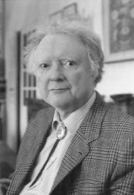
The principle of rheonomy was introduced by D’Auria and the present author in a paper of 1979 [22], formalizing a previous idea of Ne’eman and Regge [23] (see Fig. 6.9). The basic motivation to introduce such a concept was the geometrical interpretation of local supersymmetry transformations at the basis of the newly found theory of supergravity, which, at that time, was less than two year old. In this respect the key problem is that supersymmetry transformations, as they were case by case found in the early construction of supersymmetric theories, look similar to gauge-transformations, yet their gauge-field ψμ, which ultimately encodes the spin 32 particles, has not a horizontal field-strength and therefore is not a proper connection on a principal fibre-bundle. To explain this point let us remind the reader of the basic structure of the supersymmetry algebras. Consider for instance the supersymmetry algebra in the maximal D = 11 dimensions (6.2.1). The supercharges Qα anticommute to the translation generators Pa and this is the key feature in all cases. It follows that horizontality of the curvatures in the directions associated with the supercharges would imply horizontality also in the directions associated with the translations. This is absurd. Indeed, as we explained at length in the first volume, translations are eventually identified, through the soldering condition, with the diffeomorphisms on the base manifold; hence they are horizontal by definition and cannot become vertical. By means of the above argument neither the supersymmetry directions can be vertical. Yet, as already observed, considering the fermionic directions of the manifold just on the same footing as the bosonic ones is equally misleading. Indeed a metric, or vielbein, theory in superspace leads to no good physics: one has too many degrees of freedom deprived of physical meaning that have to be got rid of. What is the outcome from this dilemma? It is a revision of the concept of horizontality and, hence, of principal connections on fibre-bundles. In its strong formulation, used so far, horizontality requires that the components of the curvatures should be zero in the vertical directions. A weaker formulation of the same idea is easily deemed of: one could just require that the vertical components should just be dependent on the horizontal ones, in particular linear combinations of the latter. This very simple idea is the principle of rheonomy.

Recalling that curvatures are essentially “derivatives” of the connections, the principle of rheonomy, which “equates” vertical derivatives to horizontal ones, is reminiscent of a very classical set of equations of mathematical analysis, namely Cauchy-Riemann equations satisfied by the real and imaginary parts of an analytic

10It must also be noted that the algebras defined by (6.4.15)–(6.4.20) and by some authors named D’Auria-Frè algebras have been discussed as a possible basis for a Chern-Simons formulation of fundamental M-theory [20]. They have also been retrieved as part of a wider set of gauge algebras by Castellani [21], using his method of extended Lie derivatives.

Fig. 6.9 Born in 1931 in Torino, Tullio Regge is probably the most famous Italian physicist of the second half of the XXth century. His first achievement, that gave him world-wide fame, dates 1957 when he was only twenty-six of age. It consists of the discovery of a subtle mathematical property of potential scattering in non-relativistic quantum mechanics, namely that the scattering amplitude can be thought of as an analytic function of the angular momentum which admits an extension to the complex plane, and that the positions of the poles determine power-law growth rates for the amplitude. Easily extended to the relativistic case, Regge poles opened a new era in scattering theory and provided the framework in which, ten years later, Veneziano introduced dual amplitudes and gave birth to String Theory. In the early 1960s, Regge introduced Regge Calculus, a simplicial formulation of General Relativity where space-time is approximated by gluing together polyhedra. Regge calculus was the first instance of discretization of a gauge theory suitable for numerical simulation, and an early relative of lattice gauge theory. Very important contributions were given by him, in collaboration with Wheeler, also to the early theory of Black-Hole perturbations. Tullio Regge received the Dannie Heineman Prize for Mathematical Physics in 1964, the Città di Como prize in 1968, the Albert Einstein Award in 1979, and the Cecil Powell Medal in 1987. In 1996 he was awarded the Dirac Medal. Full Professor of Relativity of Torino University since 1961, he was member of the Institute of Advanced Studies in Princeton from the early sixties to 1979, when he resumed his chair in Torino. Elected to the European Parliament in 1989, when he finished his term in 1995, he was called on a special chair by the Politecnico di Torino, where he taught until his retirement. Tullio Regge is also full member of the Accademia dei Lincei and a public figure in Italy for his frequent participation to TV debates on a variety of problems ranging from Energetics to Bioethics. He is also an appreciated writer of quite original popularizing books and articles

Fig. 6.10 The principle of rheonomy is reminiscent of the Cauchy-Riemann equations satisfied by the real and imaginary parts of analytic functions. Hence it encodes a sort of analyticity condition for the superconnections that constitute the field content of supergravity theories

In the suggested analogy, horizontal directions correspond to the real axis x, while the role of vertical ones is played by the imaginary axis y. Furthermore the real part u(x, y) corresponds to the bosonic fields, while the imaginary part v(x, y) corresponds to the fermionic ones. Indeed in order to respect the Bose/Fermi grading, vertical components of the curvatures can be restricted to be linear functions of the horizontal ones only by relating the vertical legs of bosonic curvatures to the horizontal ones of fermionic curvatures and vice-versa. The idea of rheonomy is graphically summarized in Fig. 6.10. The analogy with Cauchy-Riemann equations and analyticity immediately suggests one important consequence of rheonomy. As it is well known, the functions u and v are not arbitrary, rather, as a consequence of the integrability of Cauchy-Riemann equations, they are harmonic functions, namely each of them satisfies Laplace equation Δu = Δv = 0. In the same way we expect that the bosonic and fermionic connections, whose curvatures are rheonomic, should obey some differential equations of the second order in the horizontal variables as a consequence of integrability of the rheonomy conditions. This is indeed the case. What are the appropriate integrability conditions in this context? The answer is simple: they are the Bianchi identities of the considered Free Differential algebra with which the rheonomic conditions must be consistent. Writing the most general rheonomic parameterization of the curvatures with arbitrary coefficients and inserting it into the Bianchi identities, one finds that all such coefficients are uniquely determined: furthermore some algebraic constraints have to be satisfied by the horizontal curvature components. These constraints are differential equations in the space-time coordinates imposed on the connection components and, in our analogy, correspond to the Laplace equation satisfied by u and v. The physical interpretation of these constraints is fascinating: they are nothing else but the appropriate field equations of supergravity theory!

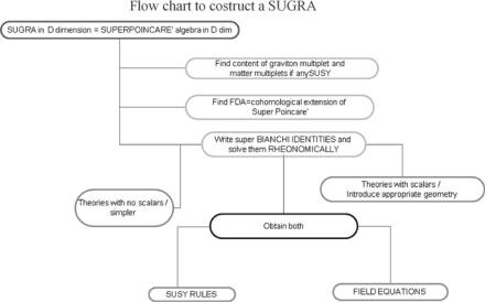
Fig. 6.11 A schematic graphical description of the steps involved in the construction of a supergravity theory

6.5.1The Flow Chart for the Construction of a Supergravity Theory

From the considerations reviewed in the previous section a well-defined schema underlying the construction of a supergravity theory emerges quite clearly. Its logic is summarized in Fig. 6.11.

There are two preliminary steps.

The first is the construction of the relevant supermultiplets, namely of the irreducible unitary representations (UIR) of the supersymmetry algebra that will be included in the theory under consideration. By definition a supermultiplet is a finite collection of unitary irreducible representations of the Poincaré Lie algebra, in other words a stack of particles labeled by their mass and their spin, which, in higher dimensions D, means the representation of the little group, SO(D − 1) for massive particles and SO(D − 2) for massless ones, to which all the available states can be assigned. This step is purely algebraic and is based on a straightforward extension to the supersymmetry algebra of the method of induced representations utilized in constructing UIR of the Poincaré Lie algebra. Knowing the supermultiplets one obtains the field content of the considered supergravity theory.

The second step consists of determining the Free Differential Algebra in which the previously fixed field content will be accommodated. According to Sullivan’s second theorem we have to consider the cohomology classes of the relevant D- dimensional super-Poincaré algebra and from that study determine the appropriate p-forms that have to be included in the list of minimal FDA generators.

Once the minimal FDA has been constructed the third step consists in its gauging. This is done by relaxing the condition that all curvatures should be zero. In this way we are able to write all the Bianchi identities and the fourth step, which is the most laborious, yet it is straightforward, consists in working out the rheonomic solution of the Bianchi identities together with its consistency conditions, coinciding with the classical field equations satisfied by the supergravity space-time fields. In the next subsection we illustrate such procedure by considering in some detail the master example of D = 11 supergravity. This is the largest possible supergravity and is thought to be the low energy effective field theory of M-theory, the so far mysterious non-perturbative theory that unifies in one more space-time dimensions all perturbative ten-dimensional superstrings.

6.5.2 Construction of D = 11 Supergravity, Alias M-Theory

In (6.4.2) we already introduced the Free Differential Algebra of M-theory and we justified its structure on the basis of Sullivan’s second theorem and of the cohomology groups of the D = 11 super-Poincaré algebra. We found that in addition to the vielbein V a , encoding the graviton degrees of freedom, the fermionic one-form ψα , encoding the degrees of freedom of a spin 32 particle, and the spin-connection ωab providing, through soldering, the propagation mechanism of the graviton, we have a three-form A[3] and a six-form A[6]. Going one step back we show here that this structure of the FDA perfectly matches with the field content of the massless multiplet of the D = 11 supersymmetry algebra which contains the spin two graviton. The structure of such a multiplet is summarized in Table 6.2 which anticipates the result. To derive such a result we argue as follows. First we construct a basis of gamma matrices well adapted to the case of massless particles propagating in a given direction, say along the 10th axis. In this case the transverse little group is SO(9) and a look at Table A.1 shows that we can represent the SO(9) Clifford

Table 6.2 Structure of the graviton multiplet in D = 11 supergravity

The five numbers given in brackets in column one are the Young labels of the corresponding irreducible representation of SO(1, 10). According to a well-established rule, for bosonic representations these labels denote the number of boxes in each row of a Young tableau which gives the symmetry of an irreducible tensor, ta1,...,an , having named n the sum of the five Young labels. For fermionic representations the Young labels are ni + 12 where once again ni give, as in the bosonic case, the description of a Young tableau. The irreducible SO(1, 10) representation is provided by an irreducible spinor tensor Taα1,...,an whose bosonic indices have the symmetry specified by the Youn tableau. All traces and gamma-traces of the irreducible spinor tensor vanish.

algebra by means of 16 × 16 symmetric matrices γ i , fulfilling the relations:

Indeed from Table A.1 we obtain the information that in d = 9 there exists only a C+ charge conjugation matrix that is symmetric and squares to the identity. When C+ is chosen to be the unit matrix, which is always possible by means of a change of basis, the gamma matrices become symmetric. Relying on this we can construct the following basis of 32 × 32 gamma matrices fulfilling the D = 11 Minkowskian Clifford algebra with the standard mostly minus metric:

With this choice the D = 11 antisymmetric charge conjugation matrix can be chosen as follows

Consider next the supersymmetry algebra as given in (6.2.1) and specialize it to the

case where the momentum vector P μ is null-like and oriented along the 10th-axis: P μ = p0(1, 0, 0, . . . , 0, 1). We obtain:

−

Imposing the Majorana condition Q = C QT on the supercharges, in the present gamma matrix basis we find the following result:

where both q and w are real operators. Hence the anticommutation relations (6.5.6) representing the supersymmetry algebra reduce to the following form:

(wα , wβ ) = 0

(qα , qβ ) = −ip0δαβ

We conclude that in a UIR massless representation of the algebra we can consistently put to zero all the operators wα and we are left with the sixteen qα which close the standard algebra of eight fermionic harmonic oscillators. Indeed we can organize the qα in two subsets of eight elements each, the former containing eight independent destruction operators, the latter containing their conjugate creation operators.

Since the sixteen operators qα transform in the spinor representation of the transverse group SO(9), we can associate them with the sixteen weights of that representation which are 4-component vectors of the following form:

all possible choices of the signs being allowed. Furthermore we can arrange matters in such a way that the creation operators are associated with the positive weights, while the destruction operators are associated with the negative ones. The positive weights can be identified with:

Let us now consider the three SO(9) representations that admit the following vectors as highest weights:

As anticipated by their names, the UIR representations of SO(1, 10) induced by the above SO(9) irreducible representations correspond to the massless graviton, to the massless gravitino and to a massless gauge particle with three antisymmetric indices, respectively. These are the particles forming the D = 11 supermultiplet as described in Table 6.2 and the number of degrees of freedom of each them is just the dimension of the corresponding SO(9) representation, in other words the number of its weights. These weights can be regarded as the possible polarizations of the corresponding massless particle propagating at the speed of light in the 10th space direction. Remains the question why precisely these representations are the content of the supermultiplet, namely why they build up an irreducible representation of the