- •Preface
- •Acknowledgements
- •Contents
- •2.1 Introduction and a Short History of Black Holes
- •2.2 The Kruskal Extension of Schwarzschild Space-Time
- •2.2.1 Analysis of the Rindler Space-Time
- •2.2.2 Applying the Same Procedure to the Schwarzschild Metric
- •2.2.3 A First Analysis of Kruskal Space-Time
- •2.3 Basic Concepts about Future, Past and Causality
- •2.3.1 The Light-Cone
- •2.3.2 Future and Past of Events and Regions
- •Achronal Sets
- •Time-Orientability
- •Domains of Dependence
- •Cauchy surfaces
- •2.4.1 Conformal Mapping of Minkowski Space into the Einstein Static Universe
- •2.4.2 Asymptotic Flatness
- •2.5 The Causal Boundary of Kruskal Space-Time
- •References
- •3.1 Introduction
- •3.2 The Kerr-Newman Metric
- •3.2.1 Riemann and Ricci Curvatures of the Kerr-Newman Metric
- •3.3 The Static Limit in Kerr-Newman Space-Time
- •Static Observers
- •3.4 The Horizon and the Ergosphere
- •The Horizon Area
- •3.5 Geodesics of the Kerr Metric
- •3.5.2 The Hamilton-Jacobi Equation and the Carter Constant
- •3.5.3 Reduction to First Order Equations
- •3.5.4 The Exact Solution of the Schwarzschild Orbit Equation as an Application
- •3.5.5 About Explicit Kerr Geodesics
- •3.6 The Kerr Black Hole and the Laws of Thermodynamics
- •3.6.1 The Penrose Mechanism
- •3.6.2 The Bekenstein Hawking Entropy and Hawking Radiation
- •References
- •4.1 Historical Introduction to Modern Cosmology
- •4.2 The Universe Is a Dynamical System
- •4.3 Expansion of the Universe
- •4.3.1 Why the Night is Dark and Olbers Paradox
- •4.3.2 Hubble, the Galaxies and the Great Debate
- •4.3.4 The Big Bang
- •4.4 The Cosmological Principle
- •4.5 The Cosmic Background Radiation
- •4.6 The New Scenario of the Inflationary Universe
- •4.7 The End of the Second Millennium and the Dawn of the Third Bring Great News in Cosmology
- •References
- •5.1 Introduction
- •5.2 Mathematical Interlude: Isometries and the Geometry of Coset Manifolds
- •5.2.1 Isometries and Killing Vector Fields
- •5.2.2 Coset Manifolds
- •5.2.3 The Geometry of Coset Manifolds
- •5.2.3.1 Infinitesimal Transformations and Killing Vectors
- •5.2.3.2 Vielbeins, Connections and Metrics on G/H
- •5.2.3.3 Lie Derivatives
- •5.2.3.4 Invariant Metrics on Coset Manifolds
- •5.2.3.5 For Spheres and Pseudo-Spheres
- •5.3 Homogeneity Without Isotropy: What Might Happen
- •5.3.1 Bianchi Spaces and Kasner Metrics
- •5.3.1.1 Bianchi Type I and Kasner Metrics
- •5.3.2.1 A Ricci Flat Bianchi II Metric
- •5.3.3 Einstein Equation and Matter for This Billiard
- •5.3.4 The Same Billiard with Some Matter Content
- •5.3.5 Three-Space Geometry of This Toy Model
- •5.4 The Standard Cosmological Model: Isotropic and Homogeneous Metrics
- •5.4.1 Viewing the Coset Manifolds as Group Manifolds
- •5.5 Friedman Equations for the Scale Factor and the Equation of State
- •5.5.1 Proof of the Cosmological Red-Shift
- •5.5.2 Solution of the Cosmological Differential Equations for Dust and Radiation Without a Cosmological Constant
- •5.5.3 Embedding Cosmologies into de Sitter Space
- •5.6 General Consequences of Friedman Equations
- •5.6.1 Particle Horizon
- •5.6.2 Event Horizon
- •5.6.3 Red-Shift Distances
- •5.7 Conceptual Problems of the Standard Cosmological Model
- •5.8 Cosmic Evolution with a Scalar Field: The Basis for Inflation
- •5.8.1 de Sitter Solution
- •5.8.2 Slow-Rolling Approximate Solutions
- •5.8.2.1 Number of e-Folds
- •5.9 Primordial Perturbations of the Cosmological Metric and of the Inflaton
- •5.9.1 The Conformal Frame
- •5.9.2 Deriving the Equations for the Perturbation
- •5.9.2.1 Meaning of the Propagation Equation
- •5.9.2.2 Evaluation of the Effective Mass Term in the Slow Roll Approximation
- •5.9.2.3 Derivation of the Propagation Equation
- •5.9.3 Quantization of the Scalar Degree of Freedom
- •5.9.4 Calculation of the Power Spectrum in the Two Regimes
- •5.9.4.1 Short Wave-Lengths
- •5.9.4.2 Long Wave-Lengths
- •5.9.4.3 Gluing the Long and Short Wave-Length Solutions Together
- •5.9.4.4 The Spectral Index
- •5.10 The Anisotropies of the Cosmic Microwave Background
- •5.10.1 The Sachs-Wolfe Effect
- •5.10.2 The Two-Point Temperature Correlation Function
- •5.10.3 Conclusive Remarks on CMB Anisotropies
- •References
- •6.1 Historical Outline and Introduction
- •6.1.1 Fermionic Strings and the Birth of Supersymmetry
- •6.1.2 Supersymmetry
- •6.1.3 Supergravity
- •6.2 Algebro-Geometric Structure of Supergravity
- •6.3 Free Differential Algebras
- •6.3.1 Chevalley Cohomology
- •Contraction and Lie Derivative
- •Definition of FDA
- •Classification of FDA and the Analogue of Levi Theorem: Minimal Versus Contractible Algebras
- •6.4 The Super FDA of M Theory and Its Cohomological Structure
- •6.4.1 The Minimal FDA of M-Theory and Cohomology
- •6.4.2 FDA Equivalence with Larger (Super) Lie Algebras
- •6.5 The Principle of Rheonomy
- •6.5.1 The Flow Chart for the Construction of a Supergravity Theory
- •6.6 Summary of Supergravities
- •Type IIA Super-Poicaré Algebra in the String Frame
- •The FDA Extension of the Type IIA Superalgebra in the String Frame
- •The Bianchi Identities
- •6.7.1 Rheonomic Parameterizations of the Type IIA Curvatures in the String Frame
- •Bosonic Curvatures
- •Fermionic Curvatures
- •6.7.2 Field Equations of Type IIA Supergravity in the String Frame
- •6.8 Type IIB Supergravity
- •SL(2, R) Lie Algebra
- •Coset Representative of SL(2, R)/O(2) in the Solvable Parameterization
- •The SU(1, 1)/U(1) Vielbein and Connection
- •6.8.2 The Free Differential Algebra, the Supergravity Fields and the Curvatures
- •The Curvatures of the Free Differential Algebra in the Complex Basis
- •The Curvatures of the Free Differential Algebra in the Real Basis
- •6.8.3 The Bosonic Field Equations and the Standard Form of the Bosonic Action
- •6.9 About Solutions
- •References
- •7.1 Introduction and Conceptual Outline
- •7.2 p-Branes as World Volume Gauge-Theories
- •7.4 The New First Order Formalism
- •7.4.1 An Alternative to the Polyakov Action for p-Branes
- •7.6 The D3-Brane: Summary
- •7.9 Domain Walls in Diverse Space-Time Dimensions
- •7.9.1 The Randall Sundrum Mechanism
- •7.9.2 The Conformal Gauge for Domain Walls
- •7.10 Conclusion on This Brane Bestiary
- •References
- •8.1 Introduction
- •8.2 Supergravity and Homogeneous Scalar Manifolds G/H
- •8.2.3 Scalar Manifolds of Maximal Supergravities in Diverse Dimensions
- •8.3 Duality Symmetries in Even Dimensions
- •8.3.1 The Kinetic Matrix N and Symplectic Embeddings
- •8.3.2 Symplectic Embeddings in General
- •8.5 Summary of Special Kähler Geometry
- •8.5.1 Hodge-Kähler Manifolds
- •8.5.2 Connection on the Line Bundle
- •8.5.3 Special Kähler Manifolds
- •8.6 Supergravities in Five Dimension and More Scalar Geometries
- •8.6.1 Very Special Geometry
- •8.6.3 Quaternionic Geometry
- •8.6.4 Quaternionic, Versus HyperKähler Manifolds
- •References
- •9.1 Introduction
- •9.2 Black Holes Once Again
- •9.2.2 The Oxidation Rules
- •Orbit of Solutions
- •The Schwarzschild Case
- •The Extremal Reissner Nordström Case
- •Curvature of the Extremal Spaces
- •9.2.4 Attractor Mechanism, the Entropy and Other Special Geometry Invariants
- •9.2.5 Critical Points of the Geodesic Potential and Attractors
- •At BPS Attractor Points
- •At Non-BPS Attractor Points of Type I
- •At Non-BPS Attractor Points of Type II
- •9.2.6.2 The Quartic Invariant
- •9.2.7.1 An Explicit Example of Exact Regular BPS Solution
- •The Metric
- •The Scalar Field
- •The Electromagnetic Fields
- •The Fixed Scalars at Horizon and the Entropy
- •The Metric
- •The Scalar Field
- •The Electromagnetic Fields
- •The Fixed Scalars at Horizon and the Entropy
- •9.2.9 Resuming the Discussion of Critical Points
- •Non-BPS Case
- •BPS Case
- •9.2.10 An Example of a Small Black Hole
- •The Metric
- •The Complex Scalar Field
- •The Electromagnetic Fields
- •The Charges
- •Structure of the Charges and Attractor Mechanism
- •9.2.11 Behavior of the Riemann Tensor in Regular Solutions
- •9.3.4 The SO(8) Spinor Bundle and the Holonomy Tensor
- •9.3.5 The Well Adapted Basis of Gamma Matrices
- •9.3.6 The so(8)-Connection and the Holonomy Tensor
- •9.3.7 The Holonomy Tensor and Superspace
- •9.3.8 Gauged Maurer Cartan 1-Forms of OSp(8|4)
- •9.3.9 Killing Spinors of the AdS4 Manifold
- •9.3.10 Supergauge Completion in Mini Superspace
- •9.3.11 The 3-Form
- •9.4.1 Maurer Cartan Forms of OSp(6|4)
- •9.4.2 Explicit Construction of the P3 Geometry
- •9.4.3 The Compactification Ansatz
- •9.4.4 Killing Spinors on P3
- •9.4.5 Gauge Completion in Mini Superspace
- •9.4.6 Gauge Completion of the B[2] Form
- •9.5 Conclusions
- •References
- •10.1 The Legacy of Volume 1
- •10.2 The Story Told in Volume 2
- •Appendix A: Spinors and Gamma Matrix Algebra
- •A.2 The Clifford Algebra
- •A.2.1 Even Dimensions
- •A.2.2 Odd Dimensions
- •A.3 The Charge Conjugation Matrix
- •A.4 Majorana, Weyl and Majorana-Weyl Spinors
- •Appendix B: Auxiliary Tools for p-Brane Actions
- •B.1 Notations and Conventions
- •Appendix C: Auxiliary Information About Some Superalgebras
- •C.1.1 The Superalgebra
- •C.2 The Relevant Supercosets and Their Relation
- •C.2.1 Finite Supergroup Elements
- •C.4 An so(6) Inversion Formula
- •Appendix D: MATHEMATICA Package NOVAMANIFOLDA
- •Coset Manifolds (Euclidian Signature)
- •Instructions for the Use
- •Description of the Main Commands of RUNCOSET
- •Structure Constants for CP2
- •Spheres
- •N010 Coset
- •RUNCOSET Package (Euclidian Signature)
- •Main
- •Spin Connection and Curvature Routines
- •Routine Curvapack
- •Routine Curvapackgen
- •Contorsion Routine for Mixed Vielbeins
- •Calculation of the Contorsion for General Manifolds
- •Calculation for Cartan Maurer Equations and Vielbein Differentials (Euclidian Signature)
- •Routine Thoft
- •AdS Space in Four Dimensions (Minkowski Signature)
- •Lie Algebra of SO(2, 3) and Killing Metric
- •Solvable Subalgebra Generating the Coset and Construction of the Vielbein
- •Killing Vectors
- •Trigonometric Coordinates
- •Test of Killing Vectors
- •MANIFOLDPROVA
- •The 4-Dimensional Coset CP2
- •Calculation of the (Pseudo-)Riemannian Geometry of a Kasner Metric in Vielbein Formalism
- •References
- •Index
5.3 Homogeneity Without Isotropy: What Might Happen |
125 |
In the case of symmetric spaces Cabe = 0 formula (5.2.100) simplifies to:
Rabcd = − |
1 |
|
2λ2 Cabi Cicd |
(5.2.101) |
5.2.3.5 For Spheres and Pseudo-Spheres
In order to illustrate the structures presented in the previous section we consider the explicit example of the spheres and pseudo-spheres. Applying the outlined procedure to this case we immediately get:
Ea = − |
2 |
|
|
dya |
|
|
||
λ 1 |
+ |
κy2 |
|
(5.2.102) |
||||
|
|
κ |
|
|
||||
|
|
|
|
|
|
|||
ωab = 2 |
|
Ea Eb |
|
|||||
λ2 |
|
This means that for spheres and pseudo-spheres the Riemann tensor is proportional to an antisymmetrized Kronecker delta:
Rabcd = |
κ |
|
λ2 δ[[ca δdb]] |
(5.2.103) |
5.3 Homogeneity Without Isotropy: What Might Happen
Having prepared the stage with our discussion of coset manifolds, among which group manifolds are a particular case, we enter the main issue of mathematical cosmology by utilizing the above developed techniques in order to construct spacetime metrics that display homogeneity with the possible addition of full or partial isotropy. The goal is that of understanding how Einstein equations turn into differential equations for the free functions fi (t) of the time variable t that parameterize such homogeneous metrics and solve them if possible. The behavior of the solutions encodes the possible scenarios of cosmic evolutions.
It is quite important to understand that the two features advocated by the Cosmological Principle, namely homogeneity and isotropy are completely independent. For this reason, in this section, we present solutions of the Einstein equations based on homogeneous but not isotropic metrics. The corresponding cosmic evolution is very different from the overall expansion motivated by Hubble Law. Without isotropy the space-like sections of the Universe not only expand or contract, but also continuously deform during time-evolution.
5.3.1 Bianchi Spaces and Kasner Metrics
A very simple way to realize a four-dimensional cosmological metric which is homogeneous without any a priori enforcement of isotropy relies on the use of the
126 |
5 Cosmology and General Relativity |
Maurer Cartan forms Ωi of a three-dimensional Lie group G3 satisfying the equation:
dΩi = tij k Ωj Ωk |
(5.3.1) |
where tij k are the structure constants of the corresponding Lie algebra G3. Assuming that the Ωi are, for instance, left-invariant we have that:
kI Ωi = 0; I = 1, 2, 3 |
(5.3.2) |
where the vector fields kI are the infinitesimal generators of the left translations. Introducing the ansatz:
dsG2 = −dt2 + Aij (t)Ωi Ωj |
(5.3.3) |
where Aij (t) is a time-dependent symmetric positive definite matrix we obtain a metric which is Lorentzian and admits the three vector fields kI as space-like translational Killing vectors. The group G3 has a transitive action on the constant time sections of such a space-time, which therefore realizes a homogeneous but a priori not isotropic cosmology.
One can insert the ansatz (5.3.3) into the Einstein equations and look for solutions with various types of matters.
The very interesting point is that in 1898 the Italian geometer Luigi Bianchi, the same who is responsible for Bianchi identities, succeeded in obtaining a complete classification of all possible three-dimensional real Lie algebras [1]. The key argument utilized by Bianchi which exploits the peculiar features of three dimensions is
the following. Given the structure constants ti |
one can define the following new |
||||
tensors: |
|
j k |
|
|
|
|
|
|
|
||
Ak = tiik |
|
|
(5.3.4) |
||
1 |
|
|
|
|
|
M i = |
|
ε j k tij k |
− δji Ak |
(5.3.5) |
|
2 |
As a consequence of its definition the matrix M i |
=i |
Mi is symmetric. In terms of |
these new objects, the vector Ak and the matrix M , the Jacobi identities reduce to |
||
the very simple condition: |
|
|
M k Ak = 0 |
|
(5.3.6) |
Hence the classification of all three-dimensional Lie algebras was reduced to the classification of solutions of (5.3.6). By means of rotations in the basis of generators the vector Ak can be oriented in a conventional direction, say the first, and the matrix M k can be diagonalized. Using this liberty the form taken by the Maurer Cartan equations of the Bianchi algebras is the following one:
dΩ1 |
= λ1 |
Ω |
2 |
Ω |
3 |
|
|
dΩ2 |
= λ2 |
Ω |
3 |
Ω |
1 |
− aΩ2 Ω1 |
(5.3.7) |
dΩ3 = λ3Ω1 Ω2 − aΩ3 Ω1 |
|
5.3 Homogeneity Without Isotropy: What Might Happen |
|
127 |
|||
Table 5.1 The classification by Bianchi of three-dimensional Lie algebras |
|
||||
|
|
|
|
|
|
Bianchi type |
a |
λ1 |
λ2 |
λ3 |
Identification |
|
|
|
|
|
|
I |
0 |
0 |
0 |
0 |
R3 |
II |
0 |
1 |
0 |
0 |
Heisenberg algebra |
III |
1 |
0 |
1 |
−1 |
|
IV |
1 |
0 |
0 |
0 |
|
V |
1 |
0 |
0 |
0 |
Solv(so(1, 3)/so(3)) |
VI0 |
0 |
1 |
−1 |
0 |
iso(1, 1) |
VIa |
a |
0 |
1 |
−1 |
|
VII0 |
0 |
1 |
1 |
0 |
iso(2) |
VIIa |
a |
0 |
1 |
1 |
so(1, 2) sl(2, R) |
VIII |
0 |
1 |
1 |
−1 |
|
IX |
0 |
1 |
1 |
1 |
so(3) |
The algebras VIa and VIIa are actually two continuous families of solvable non-isomorphic Lie algebras, distinguished by the value of the parameter a. Some of the Bianchi algebras can be identified with other well known, simple or solvable Lie algebras. Bianchi IX and Bianchi VIII are simple and correspond to the two possible real sections, respectively compact and non-compact, of the unique complex Lie algebra A1. Bianchi VII0 is the Lie algebra of the Euclidian group of the plane E2 iso(2), while Bianchi VI0 is the Poincaré Lie algebra in two dimensions iso(1, 1). Bianchi I is just the translation algebra R3, while Bianchi II is the Heisenberg algebra in two dimension. Finally according to a general theorem every non-compact simple coset manifold G/H, where H is a maximally compact subgroup, is metrically equivalent to a solvable group manifold exp Solv where the corresponding solvable Lie algebra Solv can be constructed from the Lie algebra G, according to a well defined procedure. Bianchi V is the solvable Lie algebra associated with the pseudo-sphere SO(1, 3)/SO(3).
and the various solutions are classified by specifying the four numbers λ1,2,3 and a. In this way Bianchi obtained the list of eleven algebras displayed in Table 5.1. An interesting class of solutions of Einstein equations is obtained by using the Abelian algebras of Bianchi type I.
5.3.1.1 Bianchi Type I and Kasner Metrics
Within the general class of Bianchi I metrics that can be written as follows:
dsBianchi2 I = −dt2 + Aij (t) dxi dxj |
(5.3.8) |
we can consider the subclass of Kasner metrics [2], defined below:
|
|
3 |
|
|
|
2 |
|
2 |
2 |
i 1 |
2p |
|
i |
|
|
dsKasner = −dt |
|
|
|
|
(5.3.9) |
||
|
+ t |
|
i dx |
|
|
=
128 |
5 Cosmology and General Relativity |
where pi are real exponents. The Vielbein description of the metric (5.3.9) is the following one:
E0 = dt; Ei = tpi dxi
which leads to the following spin connection
ω0i = 1 pi Ei ; ωij = 0
t
and curvature 2-form: |
|
|
|
||
1 |
|
1 |
|
||
R0i = |
|
pi (pi − 1)E0 Ei ; |
Rij = |
|
pi pj Ei Ej |
t2 |
t2 |
yielding the following Ricci tensor (in flat indices):
(5.3.10)
(5.3.11)
(5.3.12)
Ric00 = |
2t2 |
|
3 |
|
|
3 |
|
3 |
|
2 pj2 |
− pj |
||||||||
|
|
1 |
|
|
|
|
|
|
|
|
|
|
j =1 |
|
j =1 |
|
|
||
|
= |
2t |
|
|
− |
|
|
|
|
Ricii |
|
1 |
pi |
21 |
|
3 |
pj |
3 |
(5.3.13) |
|
2 |
|
j =1 |
||||||
|
|
|
|
|
|
|
|
|
|
Ricab = 0 |
if a = b |
|
|
|
|
It follows that the Kasner metric is a solution of vacuum Einstein equations, namely it is Ricci flat whenever the exponent pi satisfies the following two algebraic equations:
3 |
3 |
pj2 = 1; |
pj = 1 |
(5.3.14) |
j =1 |
j =1 |
|
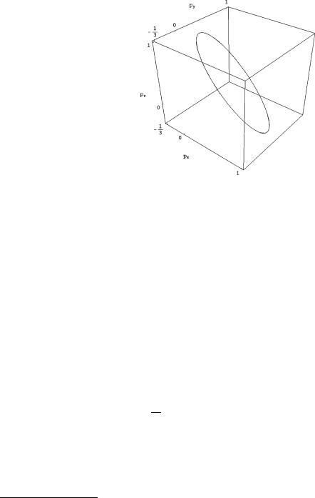
Geometrically the locus singled out by (5.3.14) is the intersection of a two-sphere with a plane and corresponds to a curve in three-dimensions that is displayed in Fig. 5.3. A parametric solution of equations is given below:
|
|
|
21 (−ω + √ |
|
+ 1) |
|
|
|
|
|
||||||||||
p1 |
|
−3ω2 + 2ω + 1 |
|
|
1 |
|
|
|||||||||||||
p2 |
|
21 ( ω |
|
√ |
|
|
|
|
|
|
|
|
1) |
|
ω |
|
|
, 1 |
(5.3.15) |
|
− |
|
− |
3ω2 |
+ |
2ω |
+ |
1 |
+ |
|
|||||||||||
|
3 |
|||||||||||||||||||
|
= |
− |
|
|
ω |
|
|
|
; |
|
− |
|
|
|
||||||
p3 |
|
|
|
|
|
|
|
|
|
|
|
|
|
|
|
|
|
|
|
|
|
|
|
|
|
|
|
|
|
|
|
|
|
|
|
|
|
|
|
|
|
Equation (5.3.15) provides just one branch of the overall solution. The other branches are obtained by applying the permutation group S3 to it and altogether they fill the curve presented in Fig. 5.3.
Any point on this curve {p1, p2, p3} yields a possible vacuum solution of Einstein equations that is named a Kasner epoch. In such Kasner epochs the destiny of the various space-dimensions is very different: some contracts, other expands, since
5.3 Homogeneity Without Isotropy: What Might Happen |
129 |
Fig. 5.3 The curve of Kasner exponents {px , py , pz} corresponding to Ricci flat metrics
the exponents pi have typically different signs. For instance a nice rational solution of the Kasner constraints is provided by:
{p1, p2, p3} = |
|
3 |
, |
3 |
, − |
3 |
|
(5.3.16) |
|
|
2 |
|
2 |
|
1 |
|
|
Let us now consider metrics of the following type: |
|
|
|
|||||
|
|
3 |
|
|
|
|
|
|
dsK2 = −dt2 + ai2(t)Ωi2 |
(5.3.17) |
|||||||
|
i=1 |
|
|
|
|
|
where Ωi are the Maurer Cartan forms of a Bianchi Lie algebra not necessarily of type I. One can draw a mechanical analogy by identifying:
hi (t) = log ai (t) |
(5.3.18) |
with the coordinates of a fictitious ball that is moving in a three-dimensional space with velocity:2
d |
|
vi (t) = dt log ai (t) |
(5.3.19) |
Kasner epochs correspond to constant velocity trajectories.
A very interesting feature arising while discussing homogeneous non isotropic solutions of Einstein equations is that of cosmic billiards. These latter are exact solutions of matter coupled higher dimensional gravity where a succession of different Kasner epochs are glued together, one after the other, in a smooth but sharp way (see
2In higher dimensional gravity theories the ball moves in n-dimensions.