Figure 2 The Gibbs Phenomenon for truncated Fourier series of a square wave

Discrete fourier transform (dft)

The computational basis of classical spectrum analysis is the Discrete Fourier Transform (DFT). The digital representation of a continuous signal y(t) in the time domain is the series

The computational basis of classical spectrum analysis is the Discrete Fourier Transform (DFT). The digital representation of a continuous signal y(t) in the time domain is the series

where is the sampling interval, S_rate is the sampling rate or sampling frequency, and N is the number of samples.

The DFT (Discrete Fourier Transform) of the discrete series y_j is given by

(6)

where . (7)

Equation (6) performs the numerical integration corresponding to the continuous integration in the definition of the Fourier transform. The values of T(f_k) represent k=N/2 discrete amplitudes spaced at discrete frequency intervals having a resolution of S_rate/N. Note, the maximum frequency of the spectrum obtained from the DFT is S_rate/2, i.e. the Nyquist frequency; thus there is no information on frequencies above half of the sampling rate. If the signal has content at frequencies above this value, aliasing will occur. To avoid this, signals are often filtered to remove frequency content above the Nyquist before they are sampled. Note that applying a digital filter after sampling will be ineffective, since aliasing will have already occurred.

From equation (7), it can be seen that reducing the sampling frequency S_rate leads to improved frequency resolution. However, in order to avoid aliasing, the sample frequency must not be reduced to less than what is required by the Nyquist criterion. The frequency resolution may be improved without changing the sample rate by increasing the number of samples taken, but this is not always possible or practical.

The size of the data array sent to the FFT, N, must be a power of two (otherwise you have a Slow Fourier Transform). Many implementations return an array of equal size, N points, but only the first N/2 are valid. The second half will simply be a mirror image of the first half. If only N/2 points are returned, they are all valid. In addition, the frequencies are usually not returned along with the amplitude information. The frequencies can be computed knowing that the bandwidth of the spectrum is from 0 to S_rate/2 Hz, and there will be N/2 equally spaced frequencies.

The fast fourier transform (fft). Spectrum analysis with fft and matlab

The fast Fourier transform (FFT) is simply a class of special algorithms which implement the discrete Fourier transform with considerable savings in computational time. It must be pointed out that the FFT is not a different transform from the DFT, but rather just a means of computing the DFT with a considerable reduction in the number of calculations required.

The typical syntax for computing FFT of a signal is FFT(x,N), where x – is the signal, x[n], you wish to transform, and N is the number of points in the FFT. N must be at least as large as the number of samples in x[n].

Let us generate sine curve within Matlab using the following commands:

Fs = 100; % sampling rate

Ts = 1/Fs; %sampling time interval, Time increment per sample

T=1;

t = 0:Ts:T; %time range

fo = 4; %frequency of the sine wave, 4Hz component

Fmax=1/Ts; %maximum frequency

df=1/T; %Frequency increment

f=0:df:Fmax; %Frequency range (Vector of frequency)

Length of a frequency vector: nf=length(f);

y = 2*sin(2*pi*fo*t); %the sine curve

Plot the sine curve in the time domain

figure(1)

plot(t,y),grid on

title('Sine Wave')

xlabel ('time (sec)')

ylabel ('output signal Y(t)')

Thus, we obtain

Figure 3 Sine wave signal

Let us use MATLAB’s built in fft command to try to recreate the frequency spectrum.

X=fft(y); %Discrete Fourier Transform

Ampl=abs(X); %use abs command to get the magnitude

figure(2)

stem(f,Ampl),grid on

xlabel('Sample Number')

ylabel('Amplitude')

title('Using the Matlab fft command')

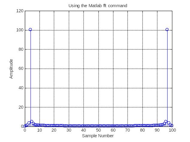
Figure 4 Fourier transform of a signal

The FFT contains information between 0 and f_s, however, we know that the sampling frequency must be at least twice the highest frequency component. Therefore, the signals spectrum should be entirely below f_s/2, the Nyquist frequency.

Recall also, that a real signal should have a transform magnitude that is symmetrical for positive and negative frequencies. Thus, instead of having a spectrum that goes from 0 to f_s, it would be more appropriate to show the spectrum from -f_s/2 to f_s/2. This can be accomplished by using Matlab’s fftshift function as the following code demonstrates.

fn=-Fmax/2:df:Fmax/2; % Normalized frequency axis

Xshift=fftshift(X);

AmplShift=abs(Xshift);

figure(3)

stem(fn,AmplShift),grid on

xlabel('Freq (Hz)')

ylabel('Amplitude')

title('Using the centeredFFT function')

Figure 5 Centered signal via fftshift command

In order to define Amplitude and phase of FFT signal he following syntax is used:

ReX0 = real(Xshift);

ImX0 = imag(Xshift);

The simulation results are represented below.

Figure 6 Amplitude and Phase for FFT of a signal

It is necessary to define some distinctive properties of Fourier Transform.

Firstly, if the signal y(t) is even then the following evenness conditions for spectrum Y( f ) come true:

where an asterisk defines complex conjugate component. It is seen that even signal possesses with even amplitude function, and phase is an odd function.

Secondly, if the signal is a real and even function of time

,

then the following conditions preserve truth for spectrum

Here the imaginary part of the spectrum is equal to zero.

Thirdly, if the signal is the real and odd function of time

,

Then the following conditions come true

In this case, the real part of the spectrum is equal to zero.