


THE HORIZONTAL BOUNDARIES |
2 |
OF THE FIRM |
|
|
|
|
|
F ew concepts in microeconomics, if any, are more fundamental to business strategy than the horizontal boundaries of the firm and the closely related topics of economies of scale and economies of scope. Economies of scale allow some firms to achieve a cost advantage over their rivals and are a key determinant of market structure and entry. Even the internal organization of a firm can be affected by the importance of realizing scale economies.
We mostly think about economies of scale as a key determinant of a firm’s horizontal boundaries, which identify the quantities and varieties of products and services that it produces. In some industries, such as microprocessors and airframe manufacturing, economies of scale are huge and a few large firms dominate. In other industries, such as web site design and shoe production, scale economies are minimal and small firms are the norm. Some industries, such as beer and computer software, have large market leaders (Anheuser-Busch, Microsoft), yet small firms (Boston Beer Company, Blizzard Entertainment) fill niches where scale economies are less important.
An understanding of the sources of economies of scale and scope is clearly critical for formulating and assessing competitive strategy. This chapter identifies the key sources of economies of scale and scope and provides approaches for assessing their importance.
DEFINITIONS
Informally, when there are economies of scale and scope, “bigger is better.” To facilitate identification and measurement, it is useful to define economies of scale and scope more precisely.
Definition of Economies of Scale
The production process for a specific good or service exhibits economies of scale over a range of output when average cost (i.e., cost per unit of output) declines over that range. If average cost (AC) declines as output increases, then the marginal cost of
61

62 • Chapter 2 • The Horizontal Boundaries of the Firm
FIGURE 2.1
A U-Shaped Average Cost Curve
AC
|
$ Per unit |
|
Average costs decline initially as fixed costs are |
|
|
spread over additional units of output. Average costs |
|
|
eventually rise as production runs up against capacity |
|
|
|
Quantity |
|
constraints. |
|
|
|
|
|
the last unit produced (MC) must be less than the average cost.1 If average cost is increasing, then marginal cost must exceed average cost, and we say that production exhibits diseconomies of scale.
An average cost curve captures the relationship between average costs and output. Economists often depict average cost curves as U-shaped, as shown in Figure 2.1, so that average costs decline over low levels of output, but increase at higher levels of output. A combination of factors may cause a firm to have U-shaped costs. A firm’s average costs may decline initially as it spreads fixed costs over increasing output. Fixed costs are insensitive to volume; they must be expended regardless of the total output. Examples of such volume-insensitive costs are manufacturing overhead expenses, such as insurance, maintenance, and property taxes. Firms may eventually see an upturn in average costs if they bump up against capacity constraints, or if they encounter coordination or other and agency problems. We will develop most of these ideas in this chapter. Coordination and agency problems are addressed in Chapters 3 and 4.
If average cost curves are U-shaped, then small and large firms would have higher costs than medium-sized firms. In reality, large firms rarely seem to be at a substantial cost disadvantage. The noted econometrician John Johnston once examined production costs for a number of industries and determined that the corresponding cost curves were closer to L-shaped than U-shaped. Figure 2.2 depicts an L-shaped cost curve. When average cost curves are L-shaped, average costs decline up to the minimum efficient scale (MES) of production and all firms operating at or beyond MES have similar average costs.
Sometimes, production exhibits U-shaped average costs in the short run, as firms that try to expand output run up against capacity constraints. In the long term, however, firms can expand their capacity by building new facilities. If each facility operates efficiently, firms can grow as large as desired without driving up average costs. This would generate the L-shaped cost curves observed by Johnston. A good example is when a cement company builds a plant in a new location. We have more to say about the distinction between shortand long-run costs later in this chapter.
Definitions • 63
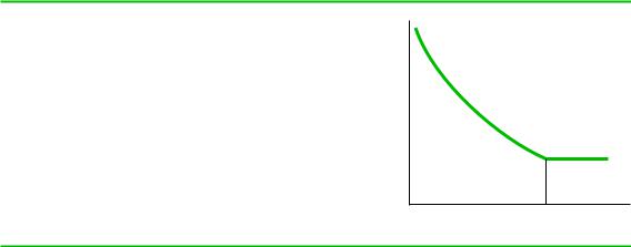
FIGURE 2.2
An L-Shaped Average Cost Curve
When capacity does not prove to be constraining, average costs may not rise as they do in a U-shaped cost curve. Output equal to or exceeding minimum efficient scale (MES) is efficient from a cost perspective.
$ Per unit
AC
MES
Quantity
Definition of Economies of Scope
Economies of scope exist if the firm achieves savings as it increases the variety of goods and services it produces. Because it is difficult to show scope economies graphically, we will instead introduce a simple mathematical formulation. Formally, let TC(Qx, Qy) denote the total cost to a single firm producing Qx units of good X and Qy units of good Y. Then a production process exhibits scope economies if
TC(Qx , Qy) , TC(Qx, 0) 1 TC(0, Qy)
This formula captures the idea that it is cheaper for a single firm to produce both goods X and Y than for one firm to produce X and another to produce Y. To provide another interpretation of the definition, note that a firm’s total costs are zero if it produces zero quantities of both products, so TC(0, 0) 5 0. Then, rearrange the preceding formula to read:
TC(Qx , Qy) 2 TC(0, Qy) , TC(Qx , 0)
This says that the incremental cost of producing Qx units of good X, as opposed to none at all, is lower when the firm is producing a positive quantity Qy of good Y.
When strategists recommend that firms “leverage core competencies” or “compete on capabilities,” they are essentially recommending that firms exploit scope economies. Tesco’s capability in warehousing and distribution gives it a cost advantage across many geographic markets. Apple’s core competency in engineering allows it to make popular cell phones, laptops, and tablet computers. Ikea’s skills in product design extends to an enormous range of home furnishing products. As these examples suggest, economies of scale and scope may arise at any point in the production process, from acquisition and use of raw inputs to distribution and retailing. Although business managers often cite scale and scope economies as justifications for growth activities and mergers, they do not always exist. In some cases, bigger may be worse! Thus, it is important to identify specific sources of scale economies and, if possible, measure their magnitude. The rest of this chapter shows how to do this.

64 • Chapter 2 • The Horizontal Boundaries of the Firm
SCALE ECONOMIES, INDIVISIBILITIES,
AND THE SPREADING OF FIXED COSTS
The most common source of economies of scale is the spreading of fixed costs over an ever-greater volume of output. Fixed costs arise when there are indivisibilities in the production process. Indivisibility simply means that an input cannot be scaled down below a certain minimum size, even when the level of output is very small.
Indivisibilities are present in nearly all production processes, and failure to recognize the associated economies of scale can cripple a firm. Web-based grocery stores such as Peapod and Webvan were once thought to have unlimited growth potential, but their enthusiasts failed to appreciate the challenge of indivisibilities. Webvan once shipped groceries from its Chicago warehouse to suburbs throughout Chicagoland. To ship to a suburb such as Highland Park, Webvan required a truck, driver, and fuel. The amount that Webvan paid for these inputs was largely independent of whether it delivered to one household or 10. Thus, these inputs represented indivisible fixed costs of serving Highland Park. Webvan was unable to generate substantial business in Highland Park (or other Illinois communities, for that matter), so it sent its trucks virtually empty. Unable to recoup warehousing costs, the company went bankrupt. Peapod faces the same problem today, but does enough business in densely populated neighborhoods in downtown Chicago to survive.
Indivisibilities can give rise to fixed costs, and hence scale and scope economies, at several different levels: the product level, the plant level, and the multiplant level. The next few subsections discuss the link between fixed costs and economies of scale at each of these levels.
Economies of Scale Due to Spreading of Product-Specific Fixed Costs
Product-specific fixed costs may include special equipment such as the cost to manufacture a special die used to make an aircraft fuselage. Fixed costs may also include research and development expenses such as the cost of developing graphics software to facilitate development of a new video game. Fixed costs may include training expenses such as the cost of a one-week training program preceding the implementation of a total quality management initiative. Fixed costs may also include setup costs such as the time and expense required to design a retailer web page.
Even a simple production process may require substantial fixed costs. The production of an aluminum can involves only a few steps. Aluminum sheets are cut to size, formed and punched into the familiar cylindrical can shape, then trimmed, cleaned, and decorated. A lid is then attached to a flange around the lip of the can, and a tab is fastened to the lid. Though the process is simple, a single line for producing aluminum cans can cost about $50 million. If the opportunity cost of tying up funds is 10 percent, the fixed costs expressed on an annualized basis amount to about $5 million per year.2
The average fixed cost of producing aluminum cans falls as output increases. To quantify this, suppose that the peak capacity of a fully automated aluminum can plant is 500 million cans annually (or about 0.5 percent of the total U.S market). The average fixed cost of operating this plant at full capacity for one year is determined by dividing the annual cost ($5,000,000) by total output (500,000,000). This works out to one cent per can. On the other hand, if the plant only operates at 25 percent of capacity,