Econometrics2011

3.18Regression Coe¢ cients

Sometimes it is useful to separate the intercept from the other regressors, and write the linear projection equation in the format

a linear equation between the centered variables y y and x x. (They are centered at their means, so are mean-zero random variables.) Because x x is uncorrelated with e; (3.32) is also a linear projection, thus by the formula for the linear projection model,

= E (x x) (x x)0 1 E (x x) y y

= var (x) 1 cov (x; y)

a function only of the covariances9 of x and y:

3.19 Regression Sub-Vectors

the coe¢ cient from the simple regression of yi on u1i:

What this means is that in the multivariate projection equation (3.38), the coe¢ cient 1 equals the projection coe¢ cient from a regression of yi on u1i; the error from a projection of x1i on the other regressors x2i: The error u1i can be thought of as the component of x1i which is not linearly explained by the other regressors. Thus the the coe¢ cient 1 equals the linear e¤ect of x1i on yi; after stripping out the e¤ects of the other variables.

There was nothing special in the choice of the variable x1i: So this derivation applies symmetrically to all coe¢ cients in a linear projection. Each coe¢ cient equals the simple regression of yi on the error from a projection of that regressor on all the other regressors. Each coe¢ cient equals the linear e¤ect of that variable on yi; after linearly controlling for all the other regressors.

3.21Omitted Variable Bias

Again, let the regressors be partitioned as in (3.35). Consider the projection of yi on x1i only. Perhaps this is done because the variables x2i are not observed. This is the equation

Notice that we have written the coe¢ cient on x1i as 1 rather than 1 and the error as ui rather than ei: This is because (3.39) is di¤erent than (3.36). Goldberger (1991) introduced the catchy labels long regression for (3.36) and short regression for (3.39) to emphasize the distinction.

Typically, 1 6= 1, except in special cases. To see this, we calculate

Observe that 1 = 1 + 2 6= 1 unless = 0 or 2 = 0: Thus the short and long regressions have di¤erent coe¢ cients on x1i: They are the same only under one of two conditions. First, if the projection of x2i on x1i yields a set of zero coe¢ cients (they are uncorrelated), or second, if the coe¢ cient on x2i in (3.36) is zero. In general, the coe¢ cient in (3.39) is 1 rather than 1: The di¤erence 2 between 1 and 1 is known as omitted variable bias. It is the consequence of omission of a relevant correlated variable.

To avoid omitted variables bias the standard advice is to include all potentially relevant variables in estimated models. By construction, the general model will be free of the omitted variables problem. Typically it is not feasible to completely follow this advice as many desired variables are not observed. In this case, the possibility of omitted variables bias should be acknowledged and discussed in the course of an empirical investigation.

3.22Best Linear Approximation

There are alternative ways we could construct a linear approximation x0 to the conditional mean m(x): In this section we show that one natural approach turns out to yield the same answer as the best linear predictor.

We start by de…ning the mean-square approximation error of x0 to m(x) as the expected squared di¤erence between x0 and the conditional mean m(x)

The function d( ) is a measure of the deviation of x0 from m(x): If the two functions are identical then d( ) = 0; otherwise d( ) > 0: We can also view the mean-square di¤erence d( ) as a densityweighted average of the function (m(x) x0 )2 ; since

d( ) = Z m(x) x0 2 fx(x)dx

Rk

where fx(x) is the marginal density of x:

We can then de…ne the best linear approximation to the conditional m(x) as the function x0 obtained by selecting to minimize d( ) :

2Rk

Similar to the best linear predictor we are measuring accuracy by expected squared error. The di¤erence is that the best linear predictor (3.19) selects to minimize the expected squared prediction error, while the best linear approximation (3.41) selects to minimize the expected squared approximation error.

Despite the di¤erent de…nitions, it turns out that the best linear predictor and the best linear approximation are identical. By the same steps as in (3.16) plus an application of conditional expectations we can …nd that

(see Exercise 3.18). Thus (3.41) equals (3.19). We conclude that the de…nition (3.41) can be viewed as an alternative motivation for the linear projection coe¢ cient.

3.23Normal Regression

Suppose the variables (y; x) are jointly normally distributed. Consider the best linear predictor of y given x

Since the error e is a linear transformation of the normal vector (y; x); it follows that (e; x) is jointly normal, and since they are jointly normal and uncorrelated (since E(xe) = 0) they are also independent (see Appendix B.9). Independence implies that

E(e j x) = E(e) = 0 and E e2 j x = E e2 = 2

which are properties of a homoskedastic linear CEF.

We have shown that when (y; x) are jointly normal, they satisfy a normal linear CEF

y = x0 + e

where

e N(0; 2)

is independent of x.

This is an alternative (and traditional) motivation for the linear CEF model. This motivation has limited merit in econometric applications since economic data is typically non-normal.

3.24Regression to the Mean

The term regression originated in an in‡uential paper by Francis Galton published in 1886, where he examined the joint distribution of the stature (height) of parents and children. E¤ectively, he was estimating the conditional mean of children’s height given their parents height. Galton discovered that this conditional mean was approximately linear with a slope of 2/3. This implies that on average a child’s height is more mediocre than his or her parent’s height. Galton called this phenomenon regression to the mean, and the label regression has stuck to this day to describe most conditional relationships.

One of Galton’s fundamental insights was to recognize that if the marginal distributions of y and x are the same (e.g. the heights of children and parents in a stable environment) then the regression slope in a linear projection is always less than one.

To be more precise, take the simple linear projection

where y equals the height of the child and x equals the height of the parent. Assume that y and x have the same mean, so that y = x = : Then from (3.33)

= (1 )

so we can write the linear projection (3.44) as

P (y j x) = (1 ) + x :

This shows that the projected height of the child is a weighted average of the population average height and the parent’s height x; with the weight equal to the regression slope : When the height distribution is stable across generations, so that var(y) = var(x); then this slope is the simple correlation of y and x: Using (3.34)

= cov (x; y) = corr(x; y): var(x)

By the properties of correlation (e.g. equation (B.7) in the Appendix), 1 corr(x; y) 1; with corr(x; y) = 1 only in the degenerate case y = x: Thus if we exclude degeneracy, is strictly less than 1.

This means that on average a child’s height is more mediocre (closer to the population average) than the parent’s.

Sir Francis Galton

Sir Francis Galton (1822-1911) of England was one of the leading …gures in late 19th century statistics. In addition to inventing the concept of regression, he is credited with introducing the concepts of correlation, the standard deviation, and the bivariate normal distribution. His work on heredity made a signi…cant intellectual advance by examing the joint distributions of observables, allowing the application of the tools of mathematical statistics to the social sciences.

A common error –known as the regression fallacy –is to infer from < 1 that the population is converging, meaning that its variance is declining towards zero. This is a fallacy because we have shown that under the assumption of constant (e.g. stable, non-converging) means and variances, the slope coe¢ cient must be less than one. It cannot be anything else. A slope less than one does not imply that the variance of y is less than than the variance of x:

Another way of seeing this is to examine the conditions for convergence in the context of equation (3.44). Since x and e are uncorrelated, it follows that

var(y) = 2 var(x) + var(e):

Then var(y) < var(x) if and only if

2 < 1 var(e) var(x)

which is not implied by the simple condition j j < 1:

The regression fallacy arises in related empirical situations. Suppose you sort families into groups by the heights of the parents, and then plot the average heights of each subsequent generation over time. If the population is stable, the regression property implies that the plots lines will converge –children’s height will be more average than their parents. The regression fallacy is to incorrectly conclude that the population is converging. The message is that such plots are misleading for inferences about convergence.

The regression fallacy is subtle. It is easy for intelligent economists to succumb to its temptation. A famous example is The Triumph of Mediocrity in Business by Horace Secrist, published in 1933. In this book, Secrist carefully and with great detail documented that in a sample of department stores over 1920-1930, when he divided the stores into groups based on 1920-1921 pro…ts, and plotted the average pro…ts of these groups for the subsequent 10 years, he found clear and persuasive evidence for convergence “toward mediocrity”. Of course, there was no discovery – regression to the mean is a necessary feature of stable distributions.

3.25Reverse Regression

Galton noticed another interesting feature of the bivariate distribution. There is nothing special about a regression of y on x: We can also regress x on y: (In his heredity example this is the best linear predictor of the height of parents given the height of their children.) This regression takes the form

This is sometimes called the reverse regression. In this equation, the coe¢ cients ; and error e are de…ned by linear projection. In a stable population we …nd that

= corr(x; y) =

= (1 ) =

which are exactly the same as in the projection of y on x! The intercept and slope have exactly the same values in the forward and reverse projections!

While this algebraic discovery is quite simple, it is counter-intuitive. Instead, a common yet mistaken guess for the form of the reverse regression is to take the equation (3.44), divide through by and rewrite to …nd the equation

suggesting that the projection of x on y should have a slope coe¢ cient of 1= instead of ; and intercept of - = rather than : What went wrong? Equation (3.46) is perfectly valid, because it is a simple manipulation of the valid equation (3.44). The trouble is that (3.46) is not a CEF nor a linear projection. Inverting a projection (or CEF) does not yield a projection (or CEF). Instead, (3.45) is a valid projection, not (3.46).

In any event, Galton’s …nding was that when the variables are standardized, the slope in both projections (y on x; and x and y) equals the correlation, and both equations exhibit regression to the mean. It is not a causal relation, but a natural feature of all joint distributions.

3.26Limitations of the Best Linear Predictor

Let’s compare the linear projection and linear CEF models.

From Theorem 3.8.1.4 we know that the CEF error has the property E(xe) = 0: Thus a linear CEF is a linear projection. However, the converse is not true as the projection error does not necessarily satisfy E(e j x) = 0:

To see this in a simple example, suppose we take a normally distributed random variable x N(0; 1) and set y = x2: Note that y is a deterministic function of x! Now consider the linear

are uncorrelated! The point is that a projection error need not be a CEF error.

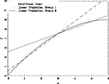
Another defect of linear projection is that it is sensitive to the marginal distribution of the regressors when the conditional mean is non-linear. We illustrate the issue in Figure 3.9 for a constructed10 joint distribution of y and x. The solid line is the non-linear CEF of y given x: The data are divided in two –Group 1 and Group 2 –which have di¤erent marginal distributions for the regressor x; and Group 1 has a lower mean value of x than Group 2. The separate linear projections of y on x for these two groups are displayed in the Figure by the dashed lines. These two projections are distinct approximations to the CEF. A defect with linear projection is that it leads to the incorrect conclusion that the e¤ect of x on y is di¤erent for individuals in the two

10 The x in Group 1 are N(2; 1) and those in Group 2 are N(4; 1); and the conditional distriubtion of y given x is

N(m(x); 1) where m(x) = 2x x2=6:

Figure 3.9: Conditional Mean and Two Linear Projections

groups. This conclusion is incorrect because in fact there is no di¤erence in the conditional mean function. The apparant di¤erence is a by-product of a linear approximation to a non-linear mean, combined with di¤erent marginal distributions for the conditioning variables.

3.27Random Coe¢ cient Model

A model which is notationally similar to but conceptually distinct from the linear CEF model is the linear random coe¢ cient model. It takes the form

y = x0

where the individual-speci…c coe¢ cient is random and independent of x. For example, if x is years of schooling and y is log wages, then is the individual-speci…c returns to schooling. If a person obtains an extra year of schooling, is the actual change in their wage. The random coe¢ cient model allows the returns to schooling to vary in the population. Some individuals might have a high return to education (a high ) and others a low return, possibly 0, or even negative.

In the linear CEF model the regressor coe¢ cient equals the regression derivative –the change in the conditional mean due to a change in the regressors, = rm(x). This is not the e¤ect on an given individual, it is the e¤ect on the population average. In contrast, in the random coe¢ cient model, the random vector = rx0 is the true causal e¤ect –the change in the response variable y itself due to a change in the regressors.

It is interesting, however, to discover that the linear random coe¢ cient model implies a linear CEF. To see this, let and denote the mean and covariance matrix of :

= E( )

= var ( )

and then decompose the random coe¢ cient as

= + u

where u is distributed independently of x with mean zero and covariance matrix : Then we can

write

E(y j x) = x0E( j x) = x0E( ) = x0

so the CEF is linear in x; and the coe¢ cients equal the mean of the random coe¢ cient . We can thus write the equation as a linear CEF

where e = x0u and u = . The error is conditionally mean zero:

E(e j x) = 0:

Furthermore

= x0 x

so the error is conditionally heteroskedastic with its variance a quadratic function of x.

Theorem 3.27.1 In the linear random coe¢ cient model y = x0 with independent of x, Ekxk2 < 1; and Ek k2 < 1; then

E(y j x) = x0 var (y j x) = x0 x

where = E( ) and = var ( ):

3.28Causal E¤ects

So far we have avoided the concept of causality, yet often the underlying goal of an econometric analysis is to uncover a causal relationship between variables. It is often of great interest to understand the causes and e¤ects of decisions, actions, and policies. For example, we may be interested in the e¤ect of class sizes on test scores, police expenditures on crime rates, climate change on economic activity, years of schooling on wages, institutional structure on growth, the e¤ectiveness of rewards on behavior, the consequences of medical procedures for health outcomes, or any variety of possible causal relationships. In each case, the goal is to understand what is the actual e¤ect on the outcome y due to a change in the input x: We are not just interested in the conditional mean or linear projection, we would like to know the actual change. The causal e¤ect is typically speci…c to an individual, and also cannot be directly observed.

For example, the causal e¤ect of schooling on wages is the actual di¤erence a person would receive in wages if we could change their level of education. The causal e¤ect of a medical treatment is the actual di¤erence in an individual’s health outcome, comparing treatment versus non-treatment. In both cases the e¤ects are individual and unobservable. For example, suppose that Jennifer would have earned $10 an hour as a high-school graduate and $20 a hour as a college graduate while George would have earned $8 as a high-school graduate and $12 as a college graduate. In this example the causal e¤ect of schooling is $10 a hour for Jennifer and $4 an hour for George. Furthermore, the causal e¤ect is unobserved as we only observe the wage corresponding to the actual outcome.

A variable x1 can be said to have a causal e¤ect on the response variable y if the latter changes when all other inputs are held constant. To make this precise we need a mathematical formulation. We can write a full model for the response variable y as