120201-7474-IJBAS-IJENS

Добавил:

Upload Опубликованный материал нарушает ваши авторские права? Сообщите нам.

Вуз:

Казахский национальный университет им. аль-Фараби

Предмет:

[НЕСОРТИРОВАННОЕ]

Файл:

p sin ( x)sin ( y ) = 0.

p sin ( x)sin ( y ) = 0.

p0 : F " − u"

.pdf

Скачиваний:

Добавлен:

08.03.2016

Размер:

134.38 Кб

Скачать

☆

1 / 21 2 > Следующая >>>

International Journal of Basic & Applied Sciences IJBAS-IJENS Vol: 12 No: 01

HOMOTOPY PERTURBATION SUMUDU TRANSFORM METHOD FOR ONE AND TWO DIMENSIONAL HOMOGENEOUS HEAT EQUATIONS

Hasan BULUT, H Mehmet BASKONUS and Seyma TULUCE

Department of Mathematics, University of Firat, 23119, Elazig-TURKEY

hbulut@firat.edu.tr , hmbaskonus@gmail.com , seymatuluce@gmail.com

Abstract

In this paper, we studied to obtain solutions of one-two dimensional homogeneous heat equations by homotopy perturbation sumudu transform method (HPSTM). We drew graphics of these equations by means of programming language Mathematica.

Keywords: Sumudu Transform Method, Homotopy Perturbation Sumudu Transform Method,

One-Two Dimensional Homogeneous Heat Equation.

1. Introduction

Sumudu Transform Method (STM) was first proposed by G. K. Watugala who was succesfully applied to various linear differential equations [1-3]. F. M. Belgacem and A. A. Karaballi introduced the fundamental properties of STM [4,5]. STM which are introduced in this paper is little known and not widely used in the literature [6-14].

Homotopy Perturbation Method (HPM) was first proposed by J.H.He [16-22]. HPM was shown that it accurately obtained solutions of homogeneous and nonhomogeneous problems [23, 24].

In this paper, we used HPSTM including STM and HPM in order to find solution of one-two dimensional homogeneous heat equations [15].

2.Analysis of the Methods

2.1Fundamental of the HPM

To illustrate the basic ideas of this method, we consider the following equation;

A(u) − f (r ) = 0,		r Ω,	(1)
with boundary condition
	∂u	r Γ,	(2)
B u,	= 0,
	∂n
where A is a general differential operator, B a boundary operator,			f (r ) a known analytical
function and Γ is the boundary of the domain Ω .

120201-7474 IJBAS-IJENS © February 2012 IJENS

I J E N S

International Journal of Basic & Applied Sciences IJBAS-IJENS Vol: 12 No: 01					7
A can be divided into two parts which are L and N ,				where L is linear and N is nonlinear.
Eq.(1) can be rewritten as following;
L (u ) + N (u ) − f (r ) = 0 , r Ω,					(3)
Homotopy perturbation structure is shown as following;
H (v, p ) = (1- p ) L (v)	- L (u	0	) + p A(v) - f	(r ) = 0,	(4)
		0
where
v(r, p): Ω × [0,1] → .					(5)
In Eq. (4), p [0,1] is an embedding parameter and u0				is the first approximation that satisfies

the boundary condition. We can assume that the solution of Eq.(4) can be written as a power series in p , as following:

v = v	+ pv + p2v	2	+ p3v + ××× ,	(6)
0	1	2	3
and the best approximation for solution is
u = lim v = v0 + v1 + v2 + v3 +L.				(7)
p→1

The convergence of series Eq.(7) has been proved by J.H. He in his paper [16]. This technique can have full advantage of the traditional perturbation techniques. Convergence rate of the series

Eq.(7) depends on the non-linear operator	A(v) . The following opinions are suggested by J.H.He
[16] .
(1) The second derivative of N (v)	with respect to v must be small because the parameter
may be relatively large, i.e., p → 1.

(2) The norm of L−1 (∂N / ∂v) must be smaller than one so that the series converges.
2.2 Fundamental of the HPSTM
To illustrate the basic ideas of this method, we consider a general linear form of partial
differantial equations;
	∂u ( x,t )	= Φ ( x,t )	∂2u ( x,t )	(8)
			∂x2
	∂t
with subject to initial condition
F ( x, 0) = f ( x ),				(9)
where f (r) is a known analytical function. The sumudu transform of Eq.(8),

120201-7474 IJBAS-IJENS © February 2012 IJENS

I J E N S

International Journal of Basic & Applied Sciences IJBAS-IJENS Vol: 12 No: 01

d 2 F ( x, u )

−

F ( x, u ) +

f ( x, 0) = 0.

uΦ

( x, u )

uΦ

( x, u )

dx2

According to HPM, we construct a homotopy in the form as following;

d 2 F

d 2 f ( x, 0)

d 2 F ( x, u )

F ( x, u )

f ( x, 0)

(1− p)

−

+ p

−

= 0

uΦ ( x, u )

where

u ( x, 0) = u0 ( x, 0) = f ( x, 0)

is initial condition of Eq.(8). Therefore, the sumudu transform of Eq.(8) is

∞

F ( x,u ) = ∑ pn Fn ( x, u ).

n=0

We can assume that the solution of Eq.(8) can be written as a power series of p,

∞

F ( x, u ) = ∑ pn Fn ( x, u )

n=0

= F0 ( x, u ) + pF1 ( x, u ) + p2 F2 ( x, u ) + p3 F3 ( x, u ) +L.

When the limit get for p →1, the solution obtain as following;

F = lim (F + pF + p2 F + p3 F +L)

→ 0 1 2 3 p 1

= F0 + F1 + F2 + F3 +L

∞

= ∑ Fn .

n=0

3. The Applications of HPSTM

3.1. Application to the One-Dimensional Homogeneous Heat Equation of HPSTM

The one-dimensional homogeneous heat equation is given by

ut = uxx − 3u , 0 < x < π , t > 0.

Initial condition for Eq.(15) is

u ( x, 0) = u0 ( x, 0) = sin ( x) .

We construct a sumudu transform for Eq.(15) as following;


S	∂u	=	1	F ( x, u ) − f ( x, 0) and	∂2u ( x, t )	=	d 2 F ( x, u )
	∂t				∂x2		dx2
			u

120201-7474 IJBAS-IJENS © February 2012 IJENS

(10)

(11)

(12)

(13)

(14)

(15)

(16)

I J E N S

International Journal of Basic & Applied Sciences IJBAS-IJENS Vol: 12 No: 01

(F ( x, u ) − f ( x, 0)) = F " − 3F

F " − 3 +

F +

sin ( x) = 0,

where is F"

d 2 F

. According to HPM, we construct a homotopy for Eq.(17);

dx2

(1− p)

+ p F −

3 +

sin ( x) = 0

− u0

F " − u0"

+ pu0" −

3 +

pF +

sin ( x) = 0.

We suppose the solution of Eq.(18) as following;

∞

F = F0 + pF1 + p2 F2 + p3 F3 +L = ∑ pn Fn ( x, u ),

n=0

∞

F " = F0" + pF1" + p2 F2" + p3 F3" +L = ∑ pn Fn" ( x, u ).

n=0

Then, by substituting Eq.(19) into Eq.(18) and rearranging

according to powers of p

obtain

F " + pF

+ p2 F "

+ p3 F

− u"

+ pu"

−

3 +

pF + p2 F + p3 F

F " + pF

+ p2 F "

+ p3 F

− u"

+ pu"

− 3 pF + −3 p2 F + −3 p3 F −

− 1 p3 F + 1 p sin ( x) = 0 u u

p0 : F0" − u0" = 0,

p1 :F" + u"	− 3F −					1	F +	1	sin ( x) = 0,
						u
1 0		0					0	u
p2 : F " − 3F −			1		F = 0,

2	1		u			1
p3 : F " − 3F −				1		F = 0,

3	2			u			2

(17)

(18)

(19)

terms, we

p sin ( x) = 0

−1 p2 F1 u

(20)

(21)

(22)

(23)

with solving Eq.(20-23)

120201-7474 IJBAS-IJENS © February 2012 IJENS

I J E N S

International Journal of Basic & Applied Sciences IJBAS-IJENS Vol: 12 No: 01

p0 : F "

− u"

= 0

= u

= sin

( x ) ,

p1 : F " + u"

− 3F −

F +

sin ( x) = 0

= ∫ ∫

−u0" +

3F0 +

F0 −

sin ( x) dx dx

0 0

= ∫ ∫

sin ( x) + 3sin ( x) +

sin ( x) −

sin ( x) dx dx

0 0

∫ ∫

4 sin ( x) dx dx

= −4 sin ( x),

: F2

− 3F1 −

F1 = 0 F2 = ∫ ∫

3F1

dx dx

0 0

= ∫ ∫

−12 sin ( x) +

(−4 sin ( x)) dx dx

0 0

= 4

3 +

sin ( x),

p3 : F "

− 3F −

F = 0

F3 = ∫ ∫

3F2

F2 dx dx

0 0

x x

= ∫ ∫

3 +

sin ( x) + 4

3 +

sin

( x) dx dx

0 0

= −4

3 +

2 sin ( x),

(24)

(25)

(26)

(27)

Because compounds of F4 , F5 , F6 ,L have very little value, we can not consider and then can take into consideration only F0 , F1 , F2 , F3 for solution by HPSTM. When we consider the series Eq.(19) and suppose p = 1 , we obtain sumudu transform of Eq.(15) as following;

120201-7474 IJBAS-IJENS © February 2012 IJENS

I J E N S

International Journal of Basic & Applied Sciences IJBAS-IJENS Vol: 12 No: 01

F ( x, u ) = F + pF + p2 F + p3 F +L

)

= lim

F + pF + p2 F + p3 F +L

p→1 (

= F0 + F1 + F2 + F3 +L

1 2

= sin ( x) −

4 sin ( x) + 4

3 +

sin

( x) − 4

sin ( x) +L

= sin ( x) 1− 4 1−

3 +

−

3 +

1 2

1 3

= sin ( x) 1− 4

−3 −

, I1

1+ 3 +

1444444442444444443

= sin ( x) 1−

+ 4u

= sin ( x)

+ 4u

Therefore we obtain sumudu transform of Eq.(15) as following;

F ( x, u )

= sin ( x)

1+ 4u

When we take inverse sumudu transform of Eq.(29) by using inverse transform table in solution of Eq.(15) by HPSTM as following;

=		u
=		1+ 4u

(28)

(29)

[4], we get

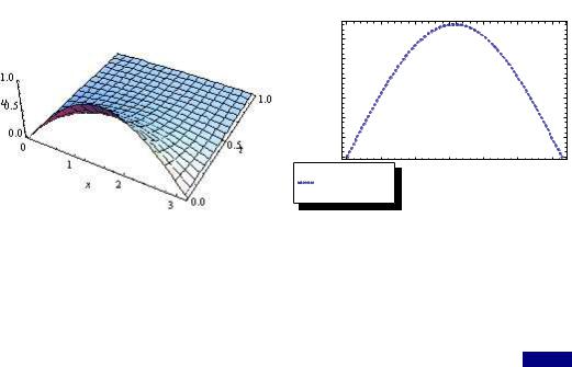
u ( x, t ) = sin ( x) e−4t .								(30)
		0.12
		0.10
		0.08
		0.06
		0.04
		0.02
		0.00
		0.0	0.5	1.0	1.5	2.0	2.5	3.0
		Exact Sol .
Figure 1. The 2D and 3D graphics for	F3	of the analytic solution u( x, t)		when t = 0.5 with initial

condition of Eq.(15) by means of HPSTM

120201-7474 IJBAS-IJENS © February 2012 IJENS

I J E N S

International Journal of Basic & Applied Sciences IJBAS-IJENS Vol: 12 No: 01

3.2. Application to the Two-Dimensional Homogeneous Heat Equation of HPSTM

The two-dimensional homogeneous heat equation is given by

= uxx + uyy ,

0 < x, y < π , t > 0.

(31)

Initial condition for Eq.(31) is

u ( x, y, 0) = u0 ( x, y, 0) = sin ( x) sin ( y).

(32)

We construct a sumudu transform for Eq.(31) as following;

S ∂u =

( x, y, u ) − f ( x, y, 0)

∂t

1 (F ( x, y, u ) − f ( x, y, 0)) = F " + F

" + F − 1

F + 1 sin ( x)sin ( y ) = 0

1 F − 1 sin ( x)sin ( y ) = F

" + F F

(33)

where are F " =

d F ( x, y,u )

d F ( x, y, u )

and F =

. According to HPM, we construct a

dx2

dy2

homotopy for Eq. (33);

(1− p) F

− u0

+ p F

+ F −

F +

sin ( x )sin ( y ) = 0

" − u0"

+ pu0"

+ p F − 1

pF + 1 p sin ( x)sin ( y ) = 0.

(34)

We suppose the solution of Eq.(34) as following;

∞

= F 0

+ p F1

+ p2 F 2 + p3 F 3

= ∑ pn F n ( x, y, u ),

n=0

∞

F " = F0" + pF1" + p2 F2" + p3 F3" +L = ∑ pn Fn" ( x, y, u ),

(35)

n=0

∞

F = F0 + pF1 + p2 F2 + p3 F3 +L = ∑ pn Fn ( x, y, u ).

n=0

Then, by substituting Eq.(35) into Eq.(34) and rearranging according to powers of p terms, we obtain

F " + pF " + p2 F " + p3 F "

− u"

+ pu"

+ p

+ p2

F 0

+ p F 1

F 2

+ p3 F 3

−

+ pF1

+ p sin ( x)sin ( y ) = 0,

p F0

+ p F2 + p F3

I J E N S

International Journal of Basic & Applied Sciences IJBAS-IJENS Vol: 12 No: 01																		13
						..		..		..		1			1
F " + pF " + p2 F " + p3 F " − u"					+ pu"	+ pF		+ p2 F		+ p3 F 2	−	1	pF	−	1	p2 F
F " + pF " + p2 F " + p3 F " − u"					+ pu"	+ pF	0	+ p2 F	1	+ p3 F 2	−		pF	−		p2 F
0	1	2	3	0	0		0		1			u	0		u		1
												u			u

p1 : F" +u" + F0 − 1 F + 1 sin(x)sin( y) = 0,
		..
1	0
1	0						u	0	u
p2 : F	" + F − 1				F = 0 ,
	..
2 1						1
2 1			u			1
p3 : F	" + F	2 − 1 F = 0 ,
	..
3						2
3				u		2
				u

with solving Eq.(36-39)

p0 : F

" − u"

= 0

F = u

= sin ( x )sin ( y ),

p1 : F " + u"

+ F 0 − 1 F + 1 sin ( x )sin ( y ) = 0

x x

= ∫ ∫ −u0

sin ( x )sin ( y ) dx dx

− F 0

−

0 0

= −2 sin ( x )sin ( y ),

x x

p : F2

+ F1

−

F1 = 0 F2 = ∫∫ − F1

dx dx

0 0

F2 = 2 1+ 1 sin ( x)sin ( y ),

3 "

x x

= ∫ ∫

p : F3

+ F 2

−

= 0 F3

− F 2

dx dx

0 0

= −2

2 sin ( x)sin ( y ),

(36)

(37)

(38)

(39)

(40)

(41)

(42)

(43)

When we consider Eq.(35) and suppose as following;

p = 1 , we obtain sumudu transform of Eq.(31) for Eq.(40-43)

I J E N S

International Journal of Basic & Applied Sciences IJBAS-IJENS Vol: 12 No: 01

F ( x, y,u) = F + pF + p2 F + p3F +L
0	1	2		3
= lim	F + pF + p2 F + p3F +L
p→1 (	0	1	2	3	)
= F0 + F1 + F2 + F3 +L
								1				1 2
= sin ( x)sin ( y) −			2sin ( x)sin ( y) + 2			1	+		sin ( x)sin ( y) − 2	1	+
= sin ( x)sin ( y) −			2sin ( x)sin ( y) + 2			1	+		sin ( x)sin ( y) − 2	1	+
								u				u

Therefore, we obtain sumudu transform of Eq.(31) as following;

(44)

sin ( x)sin ( y) +L.

F ( x, y, u ) = sin ( x)sin ( y ) 1− 2 + 2 1+

− 2 1+

= sin ( x )sin ( y ) 1− 2 + 2

1 +

−1−

−1 −

1444442444443

I = 1+

−1−

2 +L =

1+ 2u

+1+

= sin ( x)sin ( y ) 1− 2 + 2

= sin ( x)sin ( y )

−1+ 2

1+ u

u 1

+ 2u

1+ 2u

2 + 2u

= sin ( x)sin ( y ) −1

= sin ( x)sin ( y )

1+ 2u

F ( x, y, u ) = sin ( x)sin ( y )

(45)

1+ 2u

When we take inverse sumudu transform of Eq.(45) by using inverse transform table in [4], we get solution of Eq.(31) by HPSTM as following;

u ( x, y, t ) = sin ( x)sin ( y )e−2t .							(46)
	0.15
	0.10
	0.05
	0.00
	0.0	0.5	1.0	1.5	2.0	2.5	3.0
	Exact Sol .
Figure 2. The 2D and 3D graphics for F3	of the analytic solution u( x, y, t)				when	y = t = 0.5 with initial

condition of Eq.(31) by means of HPSTM

I J E N S

International Journal of Basic & Applied Sciences IJBAS-IJENS Vol: 12 No: 01

4. Conclusion

In this paper, we showed that the analytical solutions of one-two dimensional homogeneous heat equations were obtained by HPSTM. Then, we drew graphics for the these equations. STM was effectively used to solve one-two dimensional homogeneous heat equation, morever, it can be applied to partial differential equations in engineering and applied sciences.

References

[1]G. K. Watugala, Sumudu Transform: a new integral transform to solve differantial equations and control engineering problems, International Journal of Mathematical Education in Science and Technology, 24(1), 35-43, 1993.

[2]G. K. Watugala, Sumudu Transform New Integral Transform to Solve Differantial Equations and Control Engineering Problems, Mathematical Engineering in Industry, 6(4), 319-329,1998.

[3]G. K. Watugala, The Sumudu Transform for Functions of Two Variables, Mathematical Engineering in Industry, 8(4), 293-302, 2002.

[4]F. M. Belgacem, and A. A. Karaballi, Sumudu Transform Fundamental Properties Investigations and Applications, Journal of Applied Mathematics and Stochastics Analysis, 2006, 1–23, (2006).

[5]F. B. M. Belgacem, A. A. Karaballi, and S. L. Kalla, Analytical Investigations of the Sumudu Transform and Applications to Integral Production Equation, Mathematical Problems in Engineering, 2003(3), 103-118, 2003.

[6]H. Eltayeb and A. Kilicman, A Note on the Sumudu Transforms and Differantial Equations, Applied Mathematical Sciences, 4(22), 1089-1098, 2010.

[7]M. A. Asiru, Sumudu Transform and The Solution of Integral Equations of Convolution Type, International Journal of Mathematical Education in Science and Technology, 32, 906-910, 2001.

[8]M. A. Asiru, Classroom note: Application of the Sumudu Transform to Discrete Dynamic Systems, International Journal of Mathematical Education in Science and Technology, 34(6), 944-949, 2003.

[9]M. A. Asiru, Further Properties of The Sumudu Transform and Its Applications, International Journal of Mathematical Education in Science and Technology, 33(3), 441-449, 2002.

[10]V. G. Gupta, Bhavna Shrama, and A. Kilicman, , A Note on Fractional Sumudu Transforms , Journal of Applied Mathematics, 9 pages, 2010.

[11]H. Eltayeb, A. Kilicman, and B. Fisher,A New Integral Transformand Associated Distributions,Integral Transforms and Special Functions, 21(5), 367-379, 2010.

[12]V. G. Gupta and B. Sharma, Application of Sumudu Transform in Reaction-Diffusion Systems and Nonlinear Waves, Applied Mathematical Sciences, 4( 9–12), 435–446, 2010.

[13]A. Kilicman, H. Eltayeb, and P. R. Agarwal, On Sumudu Transform and System of Differantial Equations, Abstract and Applied Analysis, 2010, 11 pages, 2010.

[14]J. Singh, D. Kumar, and Sushila, Homotopy Perturbation Sumudu Transform Method for Nonlinear Equations, Adv. Theor. Mech., 4(4), 165-175, 2011.

[15]A. Wazwaz, Partial Differantial Equations: Methods and Applications, USA, (2002).

[16]J. H. He, A coupling method a homotopy technique and a perturbation technique

for non-linear problems, Int J Non-Linear Mech 35 (2000), 37–43, 2000.

[17] J.H. He, Some asymptotic methods for strongly nonlinear equations, International

I J E N S

1 / 21 2 > Следующая >>>

Соседние файлы в предмете [НЕСОРТИРОВАННОЕ]

#
24.03.201515.72 Кб151178_osymsha_4_docx_tablitsa (3).docx
#
24.03.201579.87 Кб271179_azirgi_baspa_isi.doc
#
24.03.2015936.62 Кб151190.pdf
#
25.11.2019904.7 Кб211192093689_ДОКЛАД ПО АНЕСТЕЗИИ.doc
#
24.12.2018216.05 Кб1311_1.docx
#
08.03.2016134.38 Кб11120201-7474-IJBAS-IJENS.pdf
#
08.03.2016110.83 Кб141257_zen_gidrometriasy.docx
#
24.03.201520.35 Кб2213-16 матан.docx
#
24.08.20194.95 Mб22813.doc
#
24.03.20152.46 Mб27133487.pdf
#
22.09.201952.52 Кб915-22.docx