Lab2 Physics, Balgabayeva S

Lab No.2: Study of kinematics and dynamics on the Atwood’s machine

Balgabayeva Sara

IS-126

IT department, International IT university, Dzhandosov str. 8a, 050040, Almaty

Abstract

We used the Atwood’s machine to study uniformly and uniformly accelerated motion of the loads. The Newton’s second law was proved in the third task of the experiment. I calculated the uncertainties using the Student’s method.

Introduction

Newton’s second law (F_net = ma) can be experimentally tested with an

apparatus known as an “Atwood’s Machine”. The Atwood’s machine was

constructed by R.G. Atwood in 1784. He used this machine to verify the

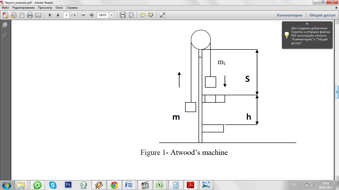
mechanical laws of motion with constant acceleration. Atwood’s machine consists of vertical stand with scale ruler. The three supporting arms are fixed on this scale ruler (the upper supporting arm with constant fixation is not shown in Fig. 1). On the stand is set up electromagnet and light pulley, which is able to rotate with insignificant friction. Over the pulley is thrown over the light string with the same mass m. Electromagnet holds the pulley with loads in the rest. Middle supporting arm is furnished by ring for taking off the overload m1. At the moment when the load m moves over the ring, the timer is switch on. The timer measures time t of uniformly motion of loads on the path h. Measuring the distance, which was passed by the load with uniformly accelerated S motion and uniformly h motion, respectively, also the time t, it is possible to prove the main laws of kinematics and dynamics for translational motion and to calculate the free fall acceleration.

Data, results and uncertainties

1. Study of uniformly motion

I set up the height of the uniformly motion of the load h=21 cm. I started the experiment and write down the readings of height and time in the table 1. I have repeated this experiment 5 times with changed height. I calculate the magnitude of the velocity by v=h/t. The results are given in the third column

of the table 1.

Table №1

№	h, m	t, sec	V, m/sec	ΔVi	ΔVi2
1	0,21	0,292	0,7191	0,0007	4,9*10^-7 0,00000049
2	0,19	0,264	0,7197	0,0013	16,9*10^-7 0,00000169
3	0,17	0,236	0,7203	0,0019	36,1*10^-7 0,00000361
4	0,15	0,209	0,7177	-0,0007	4,9*10^-7 0,00000049
5	0,13	0,181	0,7182	-0,0002	0,4*10^-7 0,00000004
6	0,11	0,153	0,7189	0,0005	2,5*10^-7 0,00000025
7	0,09	0,125	0,72	0,0016	25.6*10^-7 0,00000256
8	0,07	0,097	0,7216	0,0032	102,4*10^-7 0,00001024
9	0,05	0,070	0,7143	-0,0041	168,1*10^-7 0,00001681
10	0,03	0,042	0,7143	-0,0041	168,1*10^-7 0,00001681

Vm =0,7184

I have calculated the arithmetic mean value V of all results and obtained the following results.

= = =0,7184

I calculated the deviation of individual measurements V_i and their

squares _i², to make them in the table №1, 5 and 6 columns.

Δ V_i = V_i – V₀ , where i=1, 2, ..., n;

I calculated the mean square error of the individual measurement:

Then the mean square error of the arithmetic mean

Absolute deviation is

_<v>

Where t_p is the Student’s coefficient; t_p =2 for n=2. I suppose that the error probability α=0.95

Relative error is

Final result for the velocity is

) m/sec

2. Study of uniformly accelerated motion

By changing the positions of upper support arm from 25 until 35, I set up distance of uniformly motion S and uniformly accelerated motion h of load. I wrote down the reading in the table №2.

I measured time of uniformly motion of load t for different distances between support arms h.

Table №2

№	h, m	S, m	t, sec	a, m/sec2	Δai	Δai2
1	0,22	0,21	0,359	0,8946	0,00173	29,93*10^-8
2	0,23	0,20	0,385	0,8921	-0,00077	59,29*10^-8
3	0,24	0,19	0,412	0,8930	0,00013	1,69*10^-8
4	0,25	0,18	0,441	0,8928	-0,00007	0,49*10^-8
5	0,26	0,17	0,472	0,8929	0,00003	0,09*10^-8
6	0,27	0,16	0,505	0,8933	0,00043	18,49*10^-8
7	0,28	0,15	0,541	0,8929	0,00003	0,09*10^-8
8	0,29	0,14	0,580	0,8928	-0,00007	9,49*10^-8
9	0,3	0,13	0,623	0,8920	-0,00087	75,69*10^-8
10	0,31	0,12	0,670	0,8923	-0,00057	32,49*10^-8
				am=0,89287

Then I calculated the acceleration a for different values of S and h.

And wrote down the reading in the table №2.

I have calculated the arithmetic mean value a_m of all results and obtained the following results.

= =

I calculated the deviation of individual measurements ∆ai and their

squares ∆ai2, to make them in the table №2, 6 and 7 columns.

Δ ai = ai – a0 , where i=1, 2, ..., n;

I have calculated the uncertainty of the experiment and obtained the following results.

Standard deviation is

Absolute deviation is

_<a>

Where t_p is the Student’s coefficient; t_p =2 for n=2. I suppose that the error probability α=0.95

Relative error is

Final result for the acceleration is

) m/sec²

3. Verification of Newton’s second law

I set up distance h of uniformly accelerated motion of load.

By changing the m1 from 30 until 40 and S from 50 to 30, measure time t of uniformly motion of load at different magnitudes of h.

I wrote down the readings in Tab.3. Calculated the acceleration a.

Then I checked the relation a1 / m1 = a2 / m2 = const, where m1, m2 are masses of overloads.

m1, kg	S, m	t, sec	a, m/sec2	a/m	Δa/m	Δ(a/m)2
0,01	0,5	1,596	0,1963	19,63	0,004	16*10^1-6
0,014	0,49	1,336	0,2745	19,6171	-0,0089	79,21*10^-6
0,018	0,48	1,166	0,3531	19,6267	0,0007	0,49*10^-6
0,022	0,47	1,043	0,4320	19,6363	0,0103	106,09*10^-6
0,026	0,46	0,950	0,5096	19,6	-0,026	676*10^-6
0,03	0,45	0,874	0,5891	19,6367	0,0107	111,49*10^-6
0,034	0,44	0,812	0,6674	19,6294	0,0034	11,56*10^-6
0,038	0,43	0,759	0,7464	19,6421	0,0161	259,21*10^-6
0,042	0,42	0,714	0,8238	19,6142	-0,0118	139,24*10^-6
0,046	0,41	0,674	0,9024	19,6173	-0,0087,	75,69*10^-6
				a/m avg = 19,6260

I have calculated the arithmetic mean value a/m_m of all results and obtained the following results.

= =

I calculated the deviation of individual measurements ∆a/m and their

squares ∆a/m², to make them in the table №2, 6 and 7 columns.

I have calculated the uncertainty of the experiment and obtained the following results.

Standard deviation is

Absolute deviation is

_<a>

Where t_p is the Student’s coefficient; t_p =2 for n=2. I suppose that the error probability α=0.95

Relative error is