speech_synthesis

Section 8.2.

Phonetic Analysis

11

ANTECEDENTS

AE2 N T IH0 S IY1 D AH0 N T S

PAKISTANI

P AE2 K IH0 S T AE1 N IY0

CHANG

CH AE1 NG

TABLE

T EY1 B AH0 L

DICTIONARY

D IH1 K SH AH0 N EH2 R IY0

TROTSKY

T R AA1 T S K IY2

DINNER

D IH1 N ER0

WALTER

W AO1 L T ER0

LUNCH

L AH1 N CH

WALTZING

W AO1 L T S IH0 NG

MCFARLAND

M AH0 K F AA1 R L AH0 N D

WALTZING(2)

W AO1 L S IH0 NG

Figure 8.6 Some sample pronunciations from the CMU Pronouncing Dictionary.

DRAFT

does not distinguish between e.g., US and us (the form US has the two pronunciations

[AH1 S] and [Y UW1 EH1 S].

The 110,000 word UNISYN dictionary, freely available for research purposes,

resolves many of these issues as it was designed specifically for synthesis (Fitt, 2002).

UNISYN gives syllabifications, stress, and some morphologi cal boundaries. Further-

more, pronunciations in UNISYN can also be read off in any of dozens of dialects of

English, including General American, RP British, Australia, and so on. The UNISYN

uses a slightly different phone set; here are some examples:

going: { g * ou }.> i ng >

antecedents: { * a n . tˆ i . s ˜ ii . d n! t }> s >

dictionary: { d * i k . sh @ . n ˜ e . r ii }

8.2.2 Names

As the error analysis above indicated, names are an important issue in speech synthe-

sis. The many types can be categorized into personal names (fi rst names and surnames),

geographical names (city, street, and other place names), and commercial names (com-

pany and product names). For personal names alone, Spiegel (2003) gives an estimate

from Donnelly and other household lists of about two million different surnames and

100,000 first names just for the United States. Two million is

a very large number; an

order of magnitude more than the entire size of the CMU dictionary. For this reason,

most large-scale TTS systems include a large name pronunciation dictionary. As we

saw in Fig. 8.6 the CMU dictionary itself contains a wide variety of names; in partic-

ular it includes the pronunciations of the most frequent 50,000 surnames from an old

Bell Lab estimate of US personal name frequency, as well as 6,000 first names.

How many names are sufficient? Liberman and Church (1992) fou nd that a

dictionary of 50,000 names covered 70% of the name tokens in 44 million words of AP

newswire. Interestingly, many of the remaining names (up to 97.43% of the tokens in

their corpus) could be accounted for by simple modifications

of these 50,000 names.

For example, some name pronunciations can be created by adding simple stress-neutral

suffixes like s or ville to names in the 50,000, producing new names as follows:

walters = walter+s lucasville = lucas+ville

abelson = abel+son

Section 8.2.

Phonetic Analysis

13

The popular decision tree model for estimating this probability P(P|L) assumes

we have a hidden alignment, which tells us which phones align with each letter. We'll

need this alignment for each word in the training set. Some letters might align to

multiple phones (e.g., x often aligns to k s), while other letters might align with no

phones at all, like the final letter of cake in the following alignment:

L: c

a

k

e

|

|

|

|

P: K EY K

One method for finding such a letter-to-phone alignment is th e semi-automatic

method of (Black et al., 1998). Their algorithm is semi-automatic because it relies

on a hand-written list of the allowable phones that can realize each letter. Here are

allowables lists for the letters c and e:

c: k ch s sh t-s

e: ih iy er ax ah eh ey uw ay ow y-uw oy aa

In order to produce an alignment for each word in the training set, we take this

allowables list for all the letters, and for each word in the training set, we find all

alignments between the pronunciation and the spelling that conform to the allowables

list. From this large list of alignments, we compute, by summing over all alignments

for all words, the total count for each letter being aligned to each phone (or multi-

phone or ). From these counts we can normalize to get for each phone pi and letter l j

a probability p(pi|l j ):

(8.15)

p(pi|l j ) =

count(pi, l j )

count(l j )

We can now take these probabilities and use the Viterbi algorithm to produce the

best (Viterbi) alignment for each word, where the probability of each alignment is just

the product of all the individual phone/letter alignments.

In this way we can produce a single good alignment A for a particular pair (P, L)

in our training set. Strictly speaking, in order to estimate P(P|L), we would need to

sum over all possible alignments like this one, as follows:

(8.16)

P(P|L) =

P(P|L, A)

A

In practice, however, we'll instead approximate the probability P(P|L) via P(P|L, A),

the probability given this one good (Viterbi) alignment A. Let us suppose that there are

m aligned phone/letter pairs in A. We approximate P(P|L, A) by independently estimat-

ing the probability of each phone pi and multiplying these m estimates, as follows:

m

(8.17)

P(P|L, A) ≈

P(pi|li, other features)

i=1

For estimating the probability of each phone pi, we'll use a decision tree. What

DRAFTfeatures should we use in this decision tree besides the aligned letter li itself? Obviously

14

Chapter 8.

Speech Synthesis

there is a final

e is a useful feature. Typically we look at the k previous letters and the

k following letters.

Another useful feature would be the correct identity of the previous phone. Know-

ing this would allow us to get some phonotactic information into our probability model.

Of course, we can't know the true identity of the previous phone, but we can approxi-

mate this by looking at the previous phone that was predicted by our model. In order to

do this, we'll need to run our decision tree left to right, generating phones one by one.

In summary, in the most common decision tree model, the probability of each

DRAFT

phone pi is estimated from a window of k previous and k following letters, as well

as the most recent k phones that were previously produced, resulting in the following

equation:

m

(8.18)

P(P|L, A) ≈

P(pi|pi−1

, li+k )

i−k

i−k

i=1

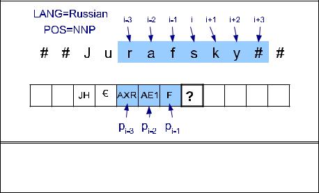
Fig. 8.7 shows a sketch of this left-to-right process, indicating the features that

a decision tree would use to decide the letter corresponding to the letter s in the word

Jurafsky. As this figure indicates, we can integrate stress predictio n into phone pre-

diction by augmenting our set of phones with stress information. We can do this by

having two copies of each vowel (e.g., AE and AE1), or possibly even the three levels

of stress AE0, AE1, and AE2, that we saw in the CMU lexicon. We'll also want to add

other features into the decision tree, including the part-of-speech tag of the word (most

part-of-speech taggers provide an estimate of the part-of-speech tag even for unknown

words) and facts such as whether the previous vowel was stressed.

In addition, grapheme-to-phoneme decision trees can also include other more so-

phisticated features. For example, we can use classes of letters (corresponding roughly

to consonants, vowels, liquids, and so on). In addition, for some languages, we need to

know features about the following word. For example French has a phenomenon called

LIAISON

liaison, in which the realization of the final phone of some words depe nds on whether

there is a next word, and whether it starts with a consonant or a vowel. For example

the French word six can be pronounced [sis] (in j'en veux six `I want six'), [siz] (six

enfants `six children'), [si] (six filles `six girls').

Finally, most synthesis systems build two separate grapheme-to-phoneme deci-

sion trees, one for unknown personal names and one for other unknown words. For

pronouncing personal names it turns out to be helpful to use additional features that

indicate which foreign language the names originally come from. Such features could

be the output of a foreign-language classifier based on lette r sequences (different lan-

guages have characteristic letter N-gram sequences).

The decision tree is a conditional classifier, computing the

phoneme string that

Section 8.3.

Prosodic Analysis

15

8.3.1 Prosodic Structure

Spoken sentences have prosodic structure in the sense that some words seem to group

naturally together and some words seem to have a noticeable break or disjuncture be-

PROSODIC

tween them. Often prosodic structure is described in terms of prosodic phrasing,

PHRASING

meaning that an utterance has a prosodic phrase structure in a similar way to it having

a syntactic phrase structure. For example, in the sentence I wanted to go to London, but

INTONATION

could only get tickets for France there seems to be two main intonation phrases, their

PHRASES

boundary occurring at the comma. Furthermore, in the first ph rase, there seems to be

INTERMEDIATE

another set of lesser prosodic phrase boundaries (often called intermediate phrases)

PHRASE

DRAFT

Section 8.3.

Prosodic Analysis

17

There is also a correlation between prosodic structure and the syntactic struc-

ture that will be introduced in Ch. 11, Ch. 12, and Ch. 14 (Price et al., 1991). Thus

robust parsers like Collins (1997) can be used to label the sentence with rough syn-

tactic information, from which we can extract syntactic features such as the size of the

biggest syntactic phrase that ends with this word (Ostendorf and Veilleux, 1994; Koehn

et al., 2000).

8.3.2 Prosodic prominence

PROMINENT

In any spoken utterance, some words sound more prominent than others. Prominent

words are perceptually more salient to the listener; speakers make a word more salient

in English by saying it louder, saying it slower (so it has a longer duration), or by

varying F0 during the word, making it higher or more variable.

We generally capture the core notion of prominence by associating a linguistic

PITCH ACCENT

marker with prominent words, a marker called pitch accent. Words which are promi-

BEAR

nent are said to bear (be associated with) a pitch accent. Pitch accent is thus part of the

phonological description of a word in context in a spoken utterance.

Pitch accent is related to stress, which we discussed in Ch. 7. The stressed

syllable of a word is where pitch accent is realized. In other words, if a speaker decides

to highlight a word by giving it a pitch accent, the accent will appear on the stressed

syllable of the word.

The following example shows accented words in capital letters, with the stressed

syllable bearing the accent (the louder, longer, syllable) in boldface:

(8.19)

I'm a little SURPRISED to hear it CHARACTERIZED as UPBEAT.

Note that the function words tend not to bear pitch accent, while most of content

words are accented. This is a special case of the more general fact that very informative

words (content words, and especially those that are new or unexpected) tend to bear

accent (Ladd, 1996; ?).

We've talked so far as if we only need to make a binary distinction between

accented and unaccented words. In fact we generally need to make more fine-grained

distinctions. For example the last accent in a phrase generally is perceived as being

more prominent than the other accents. This prominent last accent is called the nuclear

NUCLEAR ACCENT

accent. Emphatic accents like nuclear accent are generally used for semantic purposes,

for example to indicate that a word is the semantic focus of the sentence (see Ch. 20)

or that a word is contrastive or otherwise important in some way. Such emphatic words

are the kind that are often written IN CAPITAL LETTERS or with **STARS** around

them in SMS or email or Alice in Wonderland; here's an example from the latter:

(8.20)

`I know SOMETHING interesting is sure to happen,' she said to herself,

Another way that accent can be more complex than just binary is that some words

can be less prominent than usual. We introduced in Ch. 7 the idea that function words

are often phonetically very reduced.

DRAFTA final complication is that accents can differ according to t he tune associated

18

Chapter

8.

Speech Synthesis

Ignoring tune for the moment, we can summarize by saying that speech synthesis

systems can use as many as four levels of prominence: emphatic accent, pitch accent,

unaccented, and reduced. In practice, however, many implemented systems make do

with a subset of only two or three of these levels.

Let's see how a 2-level system would work. With two-levels, pitch accent pre-

diction is a binary classification task, where we are given a w ord and we have to decide

whether it is accented or not.

Since content words are very often accented, and function words are very rarely

DRAFTcent on the left. But the many exceptions to these rules make accent prediction in noun

accented, the simplest accent prediction system is just to accent all content words and

no function words. In most cases better models are necessary.

In principle accent prediction requires sophisticated semantic knowledge, for

example to understand if a word is new or old in the discourse, whether it is being used

contrastively, and how much new information a word contains. Early models made use

of sophisticated linguistic models of all of this information (Hirschberg, 1993). But

Hirschberg and others showed better prediction by using simple, robust features that

correlate with these sophisticated semantics.

For example, the fact that new or unpredictable information tends to be accented

can be modeled by using robust features like N-grams or TF*IDF (Pan and Hirschberg,

2000; Pan and McKeown, 1999). The unigram probability of a word P(wi) and its

bigram probability P(wi|wi−1), both correlate with accent; the more probable a word,

the less likely it is to be accented. Similarly, an information-retrieval measure known as

TF*IDF

TF*IDF (Term-Frequency/Inverse-Document Frequency; see Ch. 21) is a useful accent

predictor. TF*IDF captures the semantic importance of a word in a particular document

d, by downgrading words that tend to appear in lots of different documents in some

large background corpus with N documents. There are various versions of TF*IDF;

one version can be expressed formally as follows, assuming Nw is the frequency of w

in the document d, and k is the total number of documents in the corpus that contain w:

(8.21)

TF*IDF(w) = Nw × log(

N

)

k

ACCENT RATIO

For words which have been seen enough times in a training set, the accent ratio

feature can be used, which models a word's individual probability of being accented.

AccentRatio(w) =

k

where N is the total number of times the word w occurred in the

N

training set, and k is the number of times it was accented (Yuan et al., 2005).

Features like part-of-speech, N-grams, TF*IDF, and accent ratio can then be

combined in a decision tree to predict accents. While these robust features work rel-

atively well, a number of problems in accent prediction still remain the subject of re-

search.

For example, it is difficult to predict which of the two words s hould be accented

in adjective-noun or noun-noun compounds. Some regularities do exist; for example

adjective-noun combinations like new truck are likely to have accent on the right word

(new TRUCK), while noun-noun compounds like TREE surgeon are likely to have ac-

compounds quite complex. For example the noun-noun compound APPLE cake has

the accent on the first word while the noun-noun compound

apple PIE or city HALL

both have the accent on the second word (Liberman and Sproat, 1992; Sproat, 1994,

Section 8.3.

Prosodic Analysis

19

1998a).

Another complication has to do with rhythm; in general speakers avoid putting

CLASH

accents too close together (a phenomenon known as clash) or too far apart (lapse).

LAPSE

Thus city HALL and PARKING lot combine as CITY hall PARKING lot (Liberman and

Prince, 1977).

Some of these rhythmic constraints can be modeled by using machine learning

techniques that are more appropriate for sequence modeling. This can be done by

running a decision tree classifier left to right through a sen tence, and using the output

DRAFT

of the previous word as a feature, or by using more sophisticated machine learning

models like Conditional Random Fields (CRFs) (Gregory and Altun, 2004).

8.3.3 Tune

Two utterances with the same prominence and phrasing patterns can still differ prosod-

TUNE

ically by having different tunes.

The tune of an utterance is the rise and fall of its

F0 over time. A very obvious example of tune is the difference between statements

and yes-no questions in English. The same sentence can be said with a final rise in F0

to indicate a yes-no-question, or a final fall in F0 to indicat e a declarative intonation.

Fig. 8.8 shows the F0 track of the same words spoken as a question or a statement.

QUESTION RISE

Note that the question rises at the end; this is often called a question rise. The falling

FINAL FALL

intonation of the statement is called a final fall .

(Hz)

250

you

know what

(Hz)

250

mean

Pitch

i

Pitch

you

know what

i

mean

50

50

0

0.922

0

0.912

Time (s)

Time (s)

Figure 8.8 The same text read as the statement You know what I mean. (on the left) and as a question You know

what I mean? (on the right). Notice that yes-no-question intonation in English has a sharp final rise in F0.

It turns out that English makes very wide use of tune to express meaning. Besides

this well known rise for yes-no questions, ann English phrase containing a list of nouns

CONTINUATION RISE

separated by commas often has a short rise called a continuation rise after each noun.

English also has characteristic contours to express contradiction, to express surprise,

and many more.

The mapping between meaning and tune in English is extremely complex, and

20

Chapter 8.

Speech Synthesis

ToBI

TOBI

One of the most widely used linguistic models of prosody is the ToBI (Tone and Break

DRAFTsentence has the declarative boundary tone L-L%. In (b), the word Marianna is spoken

Indices) model (Silverman et al., 1992; Beckman and Hirschberg, 1994; Pierrehumbert,

1980; Pitrelli et al., 1994). ToBI is a phonological theory of intonation which models

prominence, tune, and boundaries. ToBI's model of prominence and tunes is based on

the 5 pitch accents and 4 boundary tones shown in Fig. 8.9.

Pitch Accents

Boundary Tones

H*

peak accent

L-L%

“final fall”: “declarative contour” of American En-

glish”

L*

low accent

L-H%

continuation rise

L*+H

scooped accent

H-H%

“question rise”: cantonical yes-no question con-

tour

L+H*

rising peak accent

H-L%

final level plateau (plateau because H- causes “up-

step” of following)

H+!H*

step down

Figure 8.9 The accent and boundary tones labels from the ToBI transcription system

for American English intonation (Beckman and Ayers, 1997; ?).

An utterance in ToBI consists of a sequence of intonational phrases, each of

BOUNDARY TONES

which ends in one of the four boundary tones. The boundary tones are used to rep-

resent the utterance final aspects of tune discussed in Sec. 8 .3.3. Each word in the

utterances can optionally be associated with one of the five t ypes of pitch accents.

Each intonational phrase consists of one or more intermediate phrase. These

phrases can also be marked with kinds of boundary tone, including the %H high ini-

tial boundary tone, which is used to mark a phrase which is particularly high in the

speakers' pitch range, as well as final phrase accents H- and L-.

In addition to accents and boundary tones, ToBI distinguishes four levels of

BREAK INDEX

phrasing, which are labeled on a separate break index tier. The largest levels of phras-

ing are the intonational phrase (break index 4) and the intermediate phrase (break index

3), and were discussed above. Break index 2 is used to mark a disjuncture or pause be-

tween words that is smaller than an intermediate phrase, while 1 is used for normal

phrase-medial word boundaries.

TIERS

Fig. 8.10 shows the tone, orthographic, and phrasing tiers of a ToBI transcrip-

tion, using the Praat program. We see the same sentence read with two different into-

nation patterns. In (a), the word Marianna is spoken with a high H* accent, and the