

Chris_Mi_handout
.pdfBraking Example
•Determine the energy expected when bringing a 3000lb vehicle to a halt from a speed of 60mph in 10 seconds
Energy = ½ * mass * V^2 = ½ * 3000/2.2 * (26.8 m/s)^2
= 489709 joules = 0.136 kW h
Using average speed of 30mph, the vehicle will travel 44 ft/second or 440 ft in 10 seconds,
Assume an average drag force of 100 lbf, drag loss is =100*4.455*440/3.28=59762 joules=0.0166 kW.h
Energy can be recovered is 0.136 - 0.0166 = 0.1194 Power (in 10 seconds) = 43kW
59
HEV Propulsion System Design
•The design requirements related to vehicle power typically specified by a customer are:
–the initial acceleration
–rated velocity on a given slope
–maximum % grade
–maximum steady state velocity
•The complete design is a complex issue involving numerous variables, constraints, considerations and judgment, which is beyond the scope of this course.
60
30

HEV Design Steps
•Power and energy requirement from the propulsion unit is determined from a given set of vehicle cruising and acceleration specifications
•Component level design:
–Electrical and Mechanical engineers design the electric motor for EV or the combination of electric motor and internal combustion engine for HEVs.
–Power electronics engineers design the power conversion unit which links the energy source with the electric motor.
–Controls engineer working in conjunction with the power electronics engineer develops the propulsion control system.
–Electrochemists and Chemical engineers design the energy source based on the energy requirement and guidelines of the vehicle manufacturer.
•Vehicle design is an iterative process; several designers have to interact with each other to meet the design goals.
61
Summary
•Vehicular forces include rolling resistance, gravitation, aerodynamic and traction force
•Traction and braking are achieved due to slip ratio on the wheel
•Vehicle dynamics can be derived from its kinetic motion
•Vehicle performance can be mathematically calculated with given traction force, or demanded traction force can be determined if a desired vehicle velocity profile is given
•HEV powertrain can be generally smaller due to the nature of electric motor used. The power splitting or combining is managed by vehicle control to maximize fuel economy and performance
•Rating of a powertrain can be determined using the vehicle data and design requirements
62
31
Solutions to Example 1
V |
|
(F |
|
) = |
K1 |
= 53.2 |
1.45×10 |
−3 F |
−0.0883 |
|||||
T |
TR |
|
K2 |
|
|
|
|
|
|
TR |
|
|||
|
|
|
|
|
|
|
|
|
|
|
|
|
||
K |
|
= |
FTR |
− gC |
|
K |
|
= |
ρ |
C A |
|
+ gC |
||
|
1 |
|
|
m |
|
0 |
|
2 |
|
2m |
0 F |
|
1 |
|
V |
= 42.45.4m/s, V = 60mph = 27m / s,t |
f |
= 1 |
tanh−1 (v |
f |
K |
1 |
/ K |
2 |
) |
T |
f |
K1 K |
|
|
|
|
||||
|
|
|
2 |
|
|
|
|
|
|
v(t) = 42.45 tanh(1.22×10⁻² t)
|
PT (t) = FTVT |
tanh( |
K1 K2 t) |
|
PT |
= |
1 ∫PT (t)dt = |
FTVT |
1 ln[cosh( K1 K2 t)] |
|
|
t f |
t f K1 K2 |
|
63
Solutions to Example 2
•(a) From the force balance equation, the tractive force is:
•(b) The instantaneous power is
•(c) The energy lost due to non-conservative forces
•(d) The kinetic energy of the vehicle is
•Therefore, the change in tractive energy is
FTR − FAD − Froll = m dvdt
FTR (t) = m dvdt + ρ2 CD AF v2 +mg(C0 +C1v2 )
= 464.88t +.02192t4 +62.78N.
PTR (t) = FTR (t) v(t)
=135.07t3 +.00637t6 +18.24t2W.
Eloss = ∫010 v(FAD + Froll )dt = ∫010 0.29055t2 (0.0219t4 +62.78)dt
=15,180J. |
|
∆KE = 1 m[v(10)2 −v(0)2 |
]= 337,677J |
2 |
|
∆eTR =15,180 +337,677 |
|
= 352,857J. |
64 |
32

Hybrid Electric Vehicles: Control,
Design, and Applications
Prof. Chris Mi
Department of Electrical and Computer Engineering
University of Michigan - Dearborn
4901 Evergreen Road, Dearborn, MI 48128 USA
email: chrismi@umich.edu
Tel: (313) 583-6434
Fax: (313)583-6336
Part 3
HEV Modeling and Simulation
2
1

Outline
•Vehicle Dynamics
•Modeling Basics
•Vehicle Performance
•Modeling Examples
•Modeling using Simplorer
3
Objectives
•After completing this session, you will be able to
–Write vehicle dynamic equations
–Setup simulation models using the dynamic equations
–Simulate vehicle performance for constant tractive force
–Simulate required tractive force for a desired vehicle velocity profile or gradeability
–Perform simulation using Ansoft Simplorer or related tool, using block diagrams
4
2
|
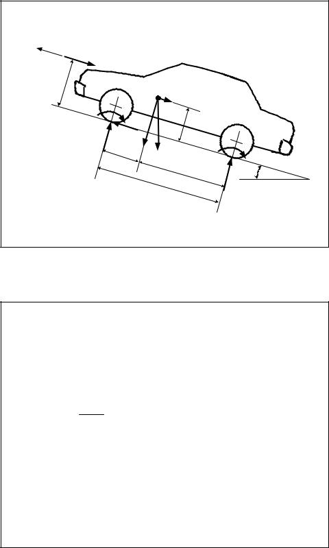
Forces Acting on a Vehicle |
|||||||
V |
F |
|
|
|
|
|
|
|
|
|
|
|
|
|
|
|
|
|
W |
|
|
|
|
|
|
|
|
h |
|
|
|
|
|
|
|
|
w |
|
|
|
|
|
|
|
|
|
|
|
|
O |
M |
|
|
|
|
|
|
|
Vg |
si |
|
|
|
|
|
|
|
|
|
n |
|
|
|
|
T |
|
|
|
α |
|
|
|
|
rf |
|
|
|
|
|
|
|
|
|
F |
|
|
h |
|
|
|
|
|
|
|
g |
||
|
|
|
|
|
t |
|
|
|
|
|
|
M |
|
|
|
|
|
|
|
|
Vg |
c |
|
|
|
|
|
|
|
|
o |
|
|
|
T |
|
|
W |
|
s |
α |
|
|
|
|
|
|
|
MVg |
rr |
|||
|
|
f |
L |
|
|
|
||
|
|
|
|
|
|
|||
|
|
|
a |
|
|
|
|
|
• Tractive force |
|
|
|
|
L |
|
α |
|
|
|
|
|
b |
|
|||
|
|
|
L |
|
|
|||
• Aerodynamic |
|
|
|
|
|
W |
||
|
|
|
|
|
|
|||
|
|
|
|
|
|
|
|
|
• Gravitational |
|
|
|
|
|
|
r |
|
|
|
|
|
|
|
|
||
• Rolling |
|
|
|
|
|
|
|
|
|
|
|
|
|
|
|
|
5 |
Dynamics of Vehicle Motion: Quarter
Vehicle Model
•The dynamic equation of motion in the tangential direction, neglecting weight shift, is
Km m dVdt = FTR − Fr
•where Km is the rotational inertia coefficient to compensate for the apparent increase in the vehicle’s mass due to the onboard rotating mass
•Typically, 1.08< Km < 1.1
6
3

Start the Modeling Process (Using
Simulink or Simplorer)
•The integration of dv/dt is speed
•The integration of v is distance
7
To Get dv/dt
•Use the vehicle dynamic equations to derive dv/dt
Km m dVdt = FTR − Fr
dVdt = (FTR − Fr ) /(Km m)
8
4
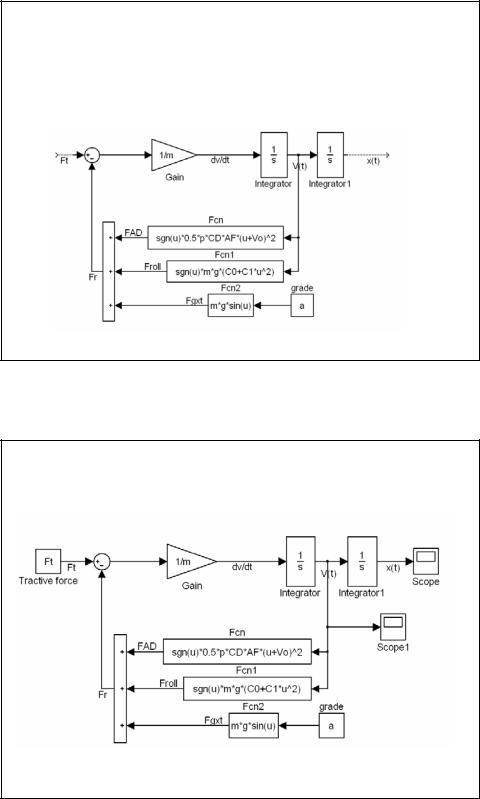
To Get Total Resistive Force Fr
•Fr = Fg+Froll+Fa
•While all forces are functions of speed
9
For Constant Tractive Force
10
5
Vehicle Dynamics Simulation Model
•Inputs to the simulation model:
–Roadway slope α
–Propulsion Force Ft
–Road Load Force Fr
•Outputs:
–Vehicle velocity V
–Distance traversed s
FTR |
|
V(t) |
|
Vehicle |
|||
|
|
||
|
Kinetics |
|
|
Grade |
Model |
S(t) |
|
|
11
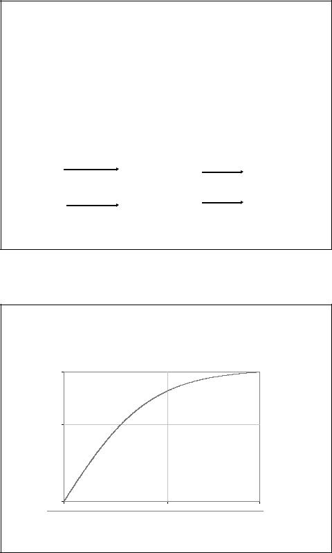
The Speed Profile with constant tractive force
|
33.80 |
|
|
Velocity (m/s) |
20.00 |
|
|
|
|
|
|
|
0 |
|
|
|
0 |
100.00 |
189.00 |
Time (s)
12
6

With 1800Nm Tractive Force
|
84.50 |
|
|
Velocity (m/s) |
50.00 |
|
|
|
|
|
|
|
0 |
|
|
|
0 |
100.00 |
189.00 |
Time (s)
13
Driving Cycles
|
100 |
|
|
Urban |
|
|
|
|
|
km/h |
|
|
|
|
|
|
|
||
|
|
|
driving |
|
|
|
|
||
50 |
|
|
|
|
|
|
|
|
|
Speed, |
|
|
|
|
|
|
|
|
|
0 0 |
|
|
|
|
|
|
|
|
|
|
200 |
400 |
600 |
800 |
|
1000 |
1200 |
1400 |
|
|
100 |
|
|
|
|
|
|
|
|
km/h |
50 |
|
|
|
Highway |
|
|
|
|
Speed, |
|
|
|
|
|
|
|
||
|
|
|
|
driving |
|
|
|
|
|
0 0 |
|
|
|
|
|
|
|
|
|
|
100 |
200 |
300 |
400 |
500 |
600 |
700 |
800 |
|
Driving time, sec.
14
7