

Chris_Mi_handout
.pdfQuestions
51

Hybrid Electric Vehicles: Control,
Design, and Applications
Prof. Chris Mi
Department of Electrical and Computer Engineering
University of Michigan - Dearborn
4901 Evergreen Road, Dearborn, MI 48128 USA
email: chrismi@umich.edu
Tel: (313) 583-6434
Fax: (313)583-6336
Part 2
HEV Fundamentals
2
1
Outline
•Vehicle Resistance
•Traction and Slip Model
•Vehicle Dynamics
•Transmission
•Vehicle Performance
•Fuel Economy and Improvements
•Braking Performance
•Power Management
•Vehicle Control
|
|
|
|
|
|
|
|
3 |
|
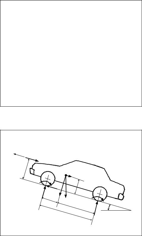
Forces Acting on a Vehicle |
|||||||
V |
F |
|
|
|
|
|
|
|
|
|
|
|
|
|
|
|
|
|
W |
|
|
|
|
|
|
|
h |
|
|
|
|
|
|
|
|
w |
|
|
|
|
|
|
|
|
|
|
|
|
|
O |
M |
|
|
|
|
|
|
|
Vg |
si |
|
|
|
|
|
|
|
|
|
n |
|
|
|
|
T |
|
|
|
α |
|
|
|
|
rf |
|
|
|
|
|
|
|
|
|
F |
|
|
h |
|
|
|
|
|
|
|
g |
||
|
|
|
|
|
t |
|
|
|
|
|
|
M |
|
|
|
|
|
|
|
|
Vg |
c |
|
|
|
|
|
|
|
|
o |
|
|
|
T |
|
|
W |
|
s |
α |
|
|
|
|
|
|
|
MVg |
rr |
|||
|
|
f |
L |
|
|
|
||
|
|
|
|
|
|
|||
• Tractive force |
|
a |
|
|
|
|
|
|
|
|
|
|
L |
|
α |
||
|
|
|
|
|
|
|
||
|
|
|
|
|
|
b |
|
|
• Aerodynamic |
|
|
|
L |
|
|
||
|
|
|
|
|
W |
|||
• Gravitational |
|
|
|
|
|
|
||
|
|
|
|
|
|
r |
||
|
|
|
|
|
|
|
||
• Rolling |
|
|
|
|
|
|
|
|
|
|
|
|
|
|
|
|
4 |
2

Grading Resistance - Gravitational
•The gravitational force, Fg depends on the slope of the roadway; it is positive when climbing a grade and is negative when descending a downgrade roadway. Where α is the grade angle with respect to the horizon, m is the total mass of the vehicle, g is the gravitational acceleration constant.
Fg = mg sinα
H
O |
M |
|
Vg s |
||
|
|
inα |
|
|
h |
α |
|
g |
|
|
|
M |
|
|
Vg |
|
|
cos |
|
|
α |
|
|
MVg
α
L
5
|
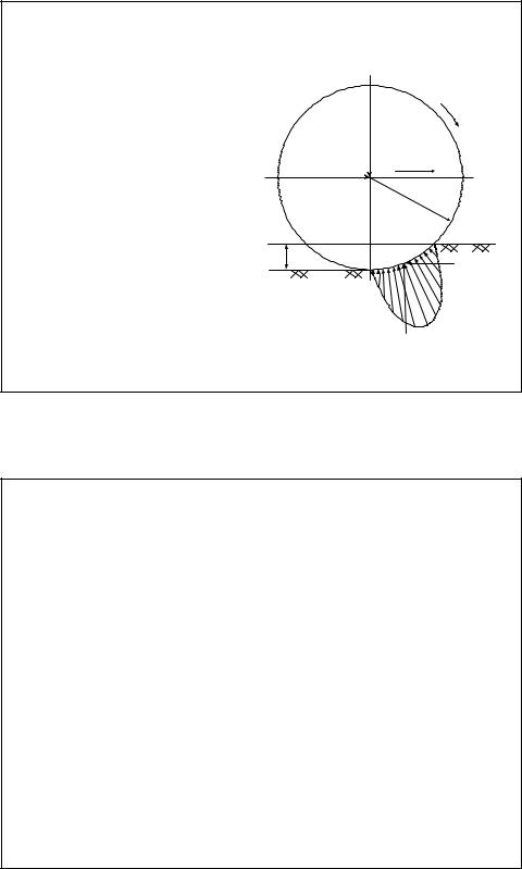
Rolling Resistance |
|
|
• On hard road surfaces |
|
|
|
– |
Caused by hysteresis of tire |
|
|
|
material |
|
P |
– |
Deflection of the carcass |
|
|
|
while the tire is rolling |
F |
Moving direction |
– |
The hysteresis causes |
|
|
|
r |
||
|
asymmetric distribution of |
|
|
|
ground reaction |
|
rd |
– |
The pressure in the leading |
|
|
|
|
||
|
half is larger than the |
|
|
|
trailing half of the contact |
|
z |
|
surface |
|
|
|
|
|
|
– |
Results in ground force |
|
a |
|
shifting forward |
|
|
|
|
|
P |
|
|
|
6 |
3
Rolling Resistance |
|
|
• On soft road surfaces |
|
|
– Caused by the deformation |
P |
|
of the ground surface |
|
|
|
|
|
– The ground reaction force |
F |
Moving direction |
almost completely shifts to |
|
|
|
r |
|
the leading half |
|
|
|
|
|
|
z |
Px |
|
|
|
|
|
Pz |
7
Rolling Resistance
• The rolling resistance force is given by
|
sgn[V ]mg(C +C V 2 ) |
if |
|
V ≠ 0 |
|
|
|
|
|
|
||||||
|
|
|
0 |
1 |
|
|
|
|
|
|
|
|
|
|
|
|
|
|
|
|
|
|
|
|
|
|
|
|
|
|
|
||
Fr |
= |
FTR − Fg |
|
if |
V = 0 |
and |
|
FTR |
− Fg |
|
|
≤ C0 mg |
||||
|
|
|
|
|||||||||||||
|
sgn(F − F )(C |
mg) |
if |
V = 0 |
and |
|
|
F |
− F |
|
|
|
> C |
mg |
||
|
|
|
|
|
||||||||||||
|
|
TR |
g 0 |
|
|
|
|
|
|
TR |
g |
|
|
0 |
|
|
|
1 |
V > 0 |
|
|
|
|
|
|
|
|
|
|
|
|
||
|
|
|
|
|
|
|
|
|
|
|
|
|
|
|||
sgn[V ] = |
V < 0 |
|
|
|
|
|
|
|
|
|
|
|
|
|||
|
|
−1 |
|
|
|
|
|
|
|
|
|
|
|
|
||
–where V is vehicle speed, FTR is the total tractive force, C0 and C1 are rolling coefficients
8
4
Typical Rolling Coefficient
• |
C0 is the maximum rolling |
Condition |
Rolling |
|
resistance at standstill |
|
coefficient C0 |
• |
0.004 < C0 < 0.02 |
Car tire on |
0.013 |
concrete or |
|||
|
(unitless) |
asphalt |
|
• |
C1 << C0 (S2/m2) |
Rolled gravel |
0.02 |
||
• |
Approximation |
Unpaved road |
0.05 |
||
|
C0 |
= 0.01 |
Field |
0.1-0.35 |
|
|
Truck tires on |
0.006-0.01 |
|||
|
|
|
V |
concrete of |
|
|
C = C |
asphalt |
|
||
|
Wheels on rails |
0.001-0.002 |
|||
|
1 |
|
0 100 |
||
|
|
|
|
|
9 |
|
|
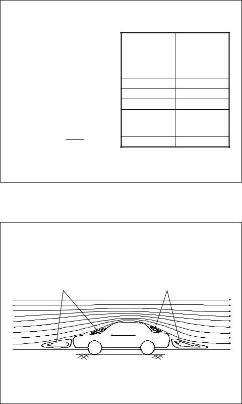
Aerodynamic Drag Force |
|||
|
|
High pressure |
Low pressure |
||
|
|
|
|
||
|
|
|
|
Moving direction |
|
|
|
|
|
|
10 |
5
Aerodynamic Drag Force FAD
•The aerodynamic drag force, FAD is the viscous resistance of the air against the motion.
–ρ: Air density
–CD : Aerodynamic drag coefficient
–AF : Equivalent frontal area of the vehicle
–Vω : Head-wind velocity
FAD = sgn[V ]{0.5ρCD AF (V +Vω )2 }
11
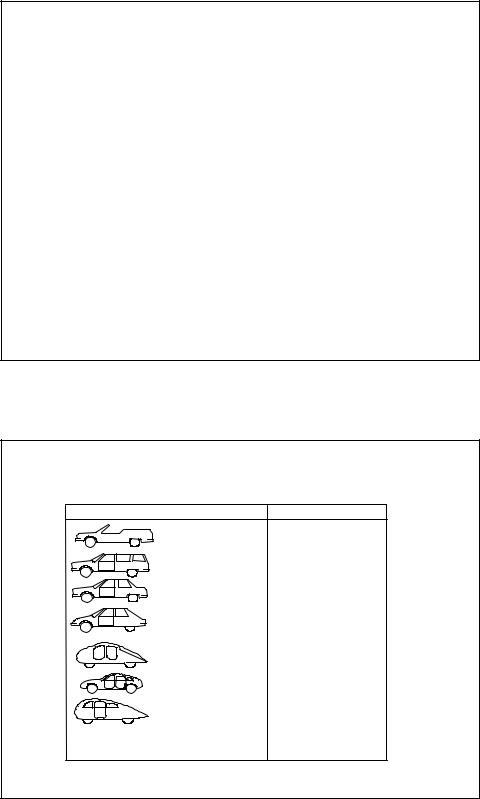
Typical Drag Coefficients
Vehicle Typ e |
Coefficient of Aerodymanic Resistance |
|
|
Open convertible |
0.5...0.7 |
Van body |
0.5...0.7 |
Ponton body |
0.4...0.55 |
Wed ge-shaped body; headlamp s and |
0.3...0.4 |
bump ers are integrated into the body , |
|
covered underbody, optimized cooling |
|
air flow. |
|
Headlamp and all wheels in |
0.2...0.25 |
body , covered underbody |
|
K-shaped (small breakway |
0.23 |
section) |
|
Optimum streamlined design |
0.15...0.20 |
Trucks, road trains |
0.8...1.5 |
Buses |
0.6...0.7 |
Streamlined buses |
0.3...0.4 |
M otorcycles |
0.6...0.7 |
12
6
Traction and Tire Slip Ratio Model
•Tractive force is introduced due to “slip” between the wheel and the vehicle linear speed
•Slip is defined as the relative difference of wheel speed and vehicle speed
•Braking force is generated by negative slip ratio
•Tractive force is proportional to adhesive coefficient
•There is a maximum tractive effect; beyond that the wheel will spin on the ground
For traction : λ = |
Vω −V |
for Braking : λ = |
Vω −V |
|
Vω |
V |
|||
|
|
13
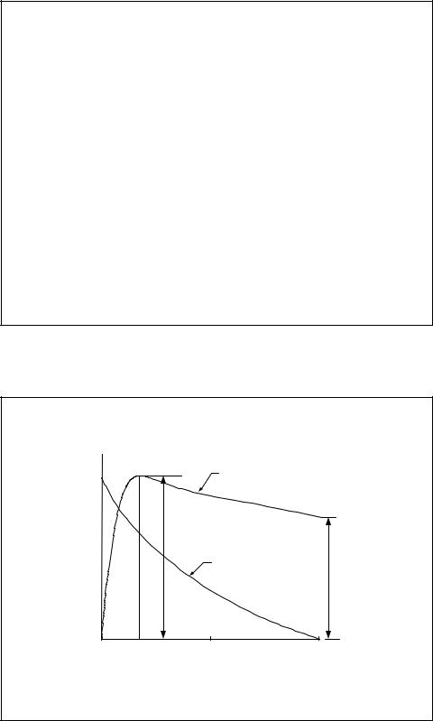
Typical Traction (adhesive) Coefficient
coefficient |
B |
Longitudinal |
|
|
|
||
A |
|
|
|
|
µp |
|
|
effort |
|
|
|
|
Lateral |
µs |
|
Tractive |
|
||
|
|
||
|
|
|
|
O0 |
15~20 |
50 |
100 % |
|
|
Slip |
|
14
7

Adhesive Coefficient for Different Road Conditions
•For almost all road conditions, braking force reaches maximum around 0.15-0.20 slip ratio.
•For traction, we need to control the torque not to exceed the maximum limited by the tire ground cohesion.
•For braking, we need to control the braking torque so that slip ratio is maintained at optimum, therefore, maximum braking effect can be achieved.
15
Dynamics of Vehicle Motion: Quarter
Vehicle Model
•The dynamic equation of motion in the tangential direction, neglecting weight shift, is
Km m dVdt = FTR − Fr
•where Km is the rotational inertia coefficient to compensate for the apparent increase in the vehicle’s mass due to the onboard rotating mass.
•Typically, 1.08< Km < 1.1
16
8

Propulsion Power
•Torque at the vehicle wheels is obtained from the power relation
P=Tωω=FtV where
Tω is the tractive torque in N-m,
ω is the angular velocity in rads/sec, Ft is in N
• The angular velocity and the vehicle speed is related by
V=ωrd
17
In Steady State
FT = mg[sinα +C0 sgn(V )]
+sgn(V )[mgC1
+ρ2 CD AF ]V 2
18
9