

3
Transmission Lines and Waveguides
Transmission lines and waveguides carry signals and power between different devices and within them. We can form many kinds of components, such as directional couplers and filters, by connecting sections of transmission lines or waveguides (see Chapters 6 and 7). Usually, lines consisting of two or more conductors are called transmission lines, and lines or wave-guiding structures having a single metal tube or no conductors at all are called waveguides. However, the use of these terms is not always consistent, and often in analysis a transmission line model is used for a waveguide (see Section 3.10).
Several types of transmission lines and waveguides have been developed for various applications. They are characterized by their attenuation, bandwidth, dispersion, purity of wave mode, power-handling capability, physical size, and applicability for integration. Dispersion means the frequency dependence of wave propagation.
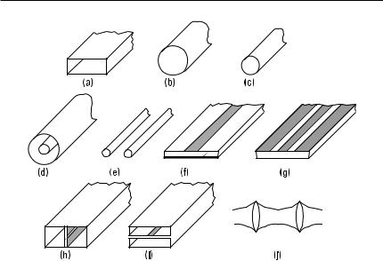
Figure 3.1 shows some types of transmission lines and waveguides, which are briefly described later. The electrical properties of the lines in Figure 3.1(a–d, f ) are explained more detailed later in this chapter; see also [1–6]. A comparison of the lines in Figure 3.1(a, d, f ) is given in Table 3.1.
A rectangular metal waveguide is a hollow metal pipe having a rectangular cross section. It has low losses and a high power-handling capability. Due to its closed structure, the fields are well isolated from the outside world. A large physical size and difficulty in integrating its components within the waveguide are the main disadvantages. The usable bandwidth for
35
36 Radio Engineering for Wireless Communication and Sensor Applications
Figure 3.1 Transmission lines and waveguides: (a) rectangular metal waveguide; (b) circular metal waveguide; (c) circular dielectric waveguide; (d) coaxial line; (e) parallel-wire line; (f) microstrip line; (g) coplanar waveguide; (h) fin line; (i) suspended stripline; and (j) quasioptical waveguide.
Table 3.1
Comparison of Some Common Lines
|
Rectangular |
|
|
Characteristic |
Waveguide |
Coaxial Line |
Microstrip Line |
|
|
|
|
Mode |
TE10 |
TEM |
Quasi-TEM |
Bandwidth |
Medium |
Broad |
Broad |
Dispersion |
Medium |
None |
Low |
Losses |
Low |
Medium |
High |
Power capability |
High |
Medium |
Low |
Size |
Large |
Medium |
Small |
Ease of fabrication |
Medium |
Medium |
Easy |
Integration |
Difficult |
Difficult |
Easy |
|
|
|
|
the pure fundamental mode TE10 is less than 1 octave. Rectangular metal waveguides are used for various applications from below 1 GHz up to 1,000 GHz and even higher frequencies.
Transmission Lines and Waveguides |
37 |
The properties of a circular metal waveguide are generally the same as those of the rectangular metal waveguide. However, the usable bandwidth for single-mode operation is even narrower, only about 25%. In an oversized circular metal waveguide, a very low-loss TE01 mode can propagate if the excitation of other modes can be prevented. (Later in this book we use the terms ‘‘rectangular waveguide’’ and ‘‘circular waveguide’’ omitting the word ‘‘metal,’’ as is often the practice in the literature.)
A circular dielectric waveguide is made of a dielectric low-loss material. Bends and other discontinuities in the line radiate easily. For example, an optical fiber is a dielectric waveguide.
A coaxial line consists of an outer and an inner conductor with circular cross sections. The space between the conductors is filled with a low-loss insulating material, such as air or Teflon. The coaxial line has a broad, singlemode bandwidth from 0 Hz to an upper limit, which depends on the dimensions of the conductors and may be as high as 60 GHz.
A parallel-wire line consists of two parallel conductors. It cannot be used at higher frequencies than in the VHF range because it has a high radiation loss at higher frequencies.
A microstrip line is made on an insulating substrate. The metal layer on the opposite side of the strip operates as a ground plane. The advantages of the microstrip line are a broad bandwidth, small size, and a good applicability for integration and mass production. The disadvantages are fairly high losses, radiation due to the open structure, and low power capability. Microstrip lines are used up to 100 GHz and even higher frequencies.
A coplanar waveguide has ground-plane conductors on both sides of a metal strip. All conductors are on the same side of the substrate. Both series and parallel components can easily be integrated with this line. Coplanar waveguides are used, for example, in monolithic integrated circuits operating at millimeter wavelengths.
A fin line is composed of a substrate in the E-plane of a rectangular (metal) waveguide. The field concentrates in a slot on the metallization of the substrate. The fin line has a low radiation loss, and components can be integrated quite easily with this line. Fin lines are used up to 200 GHz.
A suspended stripline has a substrate in the H-plane of a rectangular waveguide. There is a metal strip on the substrate.
A quasioptical waveguide is made of focusing lenses or mirrors, which maintain the energy in a beam in free space. Quasioptical waveguides are used from about 100 GHz up to infrared waves. Other lines become lossy and difficult to fabricate at such high frequencies.

38 Radio Engineering for Wireless Communication and Sensor Applications
3.1Basic Equations for Transmission Lines and Waveguides
The Helmholtz equation (2.52) is valid in the sourceless medium of a transmission line or a waveguide. Let us assume that a wave is propagating in a uniform line along the z direction. Now, the Helmholtz equation is separable so that a solution having a form of f (z ) g (x , y ) can be found. The z -dependence of the field has a form of e −gz. Thus, the electric field may be written as
E = E (x , y , z ) = g(x , y ) e −gz |
(3.1) |
where g(x , y ) is the field distribution in the transverse plane. By setting this to the Helmholtz equation, we get
|
=2 E = =2 |
E + ∂2 E |
= =2 |
E + g2 E = −v2meE |
(3.2) |
|
xy |
∂z 2 |
xy |
|
|
|
|
|
|
|
|
where =2 |
includes the partial derivatives of =2 with respect to x and y . |
||||
xy |
|
|
|
|
|
Because similar equations can be derived for the magnetic field, the partial differential equations applicable for all uniform lines are
=2 |
|
E = −( g 2 |
+ v 2me ) E |
(3.3) |
xy |
|
|
|
|
=2 |
H = −( g2 |
+ v2me) H |
(3.4) |
|
xy |
|
|
|
|
At first, the longitudinal or z -component of the electric or magnetic field is solved using the boundary conditions set by the structure of the line. When Ez or Hz is known, the x - and y -components of the fields may be solved from Maxwell’s III and IV equations. Equation = × E = −jvmH may be divided into three parts:
∂Ez /∂y + g Ey = −jvmHx
−gEx − ∂Ez /∂x = −jvmHy
∂Ey /∂x − ∂Ex /∂y = −jvmHz
Correspondingly, = × H = jve E is divided into three parts:
Transmission Lines and Waveguides |
39 |
∂Hz /∂y + gHy = jveEx
−g Hx − ∂Hz /∂x = jveEy
∂Hy /∂x − ∂Hx /∂y = jve Ez
From these, the transverse components Ex , Ey , Hx , and Hy are solved as functions of the longitudinal components Ez and Hz :
|
|
|
|
|
−1 |
|
|
|
|
∂Ez |
|
|
∂Hz |
|
|
||||
Ex = |
|
|
|
|
|
|
S |
g |
∂x |
+ jvm |
∂y D |
(3.5) |
|||||||
g2 + v2me |
|||||||||||||||||||
|
|
|
|
|
|
|
|||||||||||||
Ey = |
|
|
|
|
1 |
|
|
|
−g |
∂Ez |
+ jvm |
∂Hz |
|
(3.6) |
|||||
g2 + v2me S |
∂y |
∂x |
D |
||||||||||||||||
|
|
|
|
|
|
|
|||||||||||||
|
|
|
|
|
1 |
|
|
|
|
|
|
|
∂Ez |
|
∂Hz |
|
|
||
Hx = |
|
|
|
|
S |
jve |
∂y |
− g |
∂x D |
(3.7) |
|||||||||
g |
2 + v 2me |
||||||||||||||||||
|
|
|
|
|
|
|
|
||||||||||||
|
|
|
|
|
−1 |
|
|
|
|
|
∂Ez |
|
∂Hz |
|
|
||||
Hy = |
|
|
|
|
S |
jve |
∂x |
+ g |
∂y D |
(3.8) |
|||||||||
g |
2 + v 2me |
||||||||||||||||||
|
|
|
|
|
|
|
|||||||||||||
In a cylindrical coordinate system, the solution of the Helmholtz equation has the form of f (z ) g (r , f ). As above, the transverse r - and f -components are calculated from the longitudinal components:
|
|
|
|
|
−1 |
|
|
|
|
|
|
∂Ez |
|
|
jvm |
∂Hz |
|
|
|
|||||
Er = |
|
|
|
|
|
|
S |
g |
|
∂r |
|
+ |
|
|
|
∂f D |
(3.9) |
|||||||
g2 + v2me |
|
|
|
|
r |
|||||||||||||||||||
|
|
|
|
|
|
|
|
|
|
|
||||||||||||||
|
|
|
|
|
1 |
|
|
|
|
|
g ∂Ez |
|
|
|
∂Hz |
|
|
|||||||
Ef = |
|
|
|
|
S− |
|
∂f |
+ jvm ∂r |
|
D |
(3.10) |
|||||||||||||
g2 + v2me |
r |
|
||||||||||||||||||||||
|
|
|
|
|
1 |
|
|
|
|
|
jve ∂Ez |
|
|
∂Hz |
|
|
|
|||||||
Hr = |
|
|
|
|
|
|
|
|
|
|
|
|
|
|
|
|
− g |
∂r D |
(3.11) |
|||||
g |
2 + v 2me |
|
S r |
|
|
|
∂f |
|||||||||||||||||
|
|
|
|
|
|
|
|
|
|
|||||||||||||||
Hf = |
|
−1 |
|
|
Sjve |
∂Ez |
+ |
g ∂Hz |
D |
(3.12) |
||||||||||||||
g2 + v2me |
|
|
∂r |
|
r |
∂f |
||||||||||||||||||
In a given waveguide at a given frequency, several field configurations may satisfy Maxwell’s equations. These field configurations are called wave