- •1. TABLE OF CONTENTS
- •2. AN INTRODUCTION TO UNIX
- •2.1 OVERVIEW
- •2.2 UNIX
- •2.2.1 Using UNIX Workstations in general:
- •2.2.2 Directories, Files, Etc.
- •2.2.3 Advanced Concepts
- •2.3 THE NETWORK
- •2.4 GOOD MANNERS
- •3. THE INTERNET
- •3.1 NETWORKS
- •3.1.1 Computer Addresses
- •3.2 NETWORK TYPES
- •3.2.1 Permanent Wires
- •3.2.2 Phone Lines
- •3.3 NETWORK PROTOCOLS
- •3.3.1 Mail Transfer Protocols
- •3.3.1.1 - Attachments
- •3.3.1.2 - Mail Lists
- •3.3.2 FTP - File Transfer Protocol
- •3.3.3 News
- •3.3.4 HTTP - Hypertext Transfer Protocol
- •3.3.5 Chat
- •3.3.6 Novell
- •3.3.7 Security
- •3.4 DATA FORMATS
- •3.4.1 HTML - Hyper Text Markup Language
- •3.4.1.1 - Publishing Web Pages
- •3.4.2 URLs
- •3.4.3 Hints
- •3.4.4 Specialized Editors
- •3.4.6 Encryption
- •3.4.7 Compression
- •3.5 PULLING ALL THE PROTOCOLS AND FORMATS TOGETHER WITH BROWSWERS
- •3.6 OTHER STUFF
- •3.6.1 Clients and Servers
- •3.6.2 Java
- •3.6.3 Javascript
- •3.6.5 Searches
- •3.6.6 ActiveX
- •3.6.7 Graphics
- •3.6.8 Animation
- •3.6.9 Video
- •3.6.10 Sounds
- •3.6.11 Other Program Files
- •3.6.12 Fancy Stuff
- •4. TEACHING WITH THE INTERNET
- •4.1 LECTURES
- •4.1.1 Equipment
- •4.1.2 Techniques
- •4.2 ON-LINE NOTES
- •4.3 ON-LINE MARKING
- •4.3.1 Web Pages
- •4.3.2 email
- •4.4 The Time-Line For My First On-Line Course (Fall 1996)
- •5. WWW and HTML
- •5.1 Why Bother?
- •5.2 Where to Find Netscape
- •5.3 How to Get Your Own Home Page
- •5.4 How to Create a file
- •5.5 Resources
- •6. A BASIC INTRODUCTION TO ‘C’
- •6.2 BACKGROUND
- •6.3 PROGRAM PARTS
- •6.4 HOW A ‘C’ COMPILER WORKS
- •6.5 STRUCTURED ‘C’ CODE
- •6.6 ARCHITECTURE OF ‘C’ PROGRAMS (TOP-DOWN)
- •6.7 CREATING TOP DOWN PROGRAMS
- •6.8.1 Objectives:
- •6.8.2 Problem Definition:
- •6.8.3 User Interface:
- •6.8.3.1 - Screen Layout (also see figure):
- •6.8.3.2 - Input:
- •6.8.3.3 - Output:
- •6.8.3.4 - Help:
- •6.8.3.5 - Error Checking:
- •6.8.3.6 - Miscellaneous:
- •6.8.4 Flow Program:
- •6.8.5 Expand Program:
- •6.8.6 Testing and Debugging:
- •6.8.7 Documentation
- •6.8.7.1 - Users Manual:
- •6.8.7.2 - Programmers Manual:
- •6.8.8 Listing of BeamCAD Program.
- •6.9 PRACTICE PROBLEMS
- •7. GUI DESIGN
- •7.1 PRACTICE PROBLEMS
- •8. AN EXAMPLE - BEAMCAD
- •9. PROGRAMMING IN JAVA
- •9.1 OVERVIEW
- •9.2 THE LANGUAGE
- •9.3 OBJECT ORIENTED PROGRAMMING
- •9.4 REFERENCES/BIBLIOGRAPHY
- •10. DATABASES
- •11. MESSAGE PASSING ON NETWORKS
- •12. MATHEMATICAL ELEMENTS OF COMPUTER GRAPHICS
- •12.1 INTRODUCTION
- •12.2 PIXELS
- •12.2.1 The Perspective Transform
- •12.3 LINE DRAWING
- •12.3.1 Hidden Lines
- •12.4 POLYGON DRAWING
- •12.5 SHADED POLYGONS
- •12.6 COLORS
- •12.6.1 Color Maps
- •12.6.1.1 - Quantization with an Octree RGB Cube
- •12.6.1.1.1 - Algorithm and Implementation
- •12.6.1.1.2 - Color Quantization Data Structures
- •12.7 DITHERING
- •12.7.1 A Model for Light Ray Reflection
- •12.7.2 A Model for Light Ray Refraction:
- •12.7.3 A Model for Specular Reflection of Point Light
- •12.8 RAY TRACING
- •12.8.1 Basic Ray Tracing Theory
- •12.8.1.1 - A Model for Diffuse Reflection of Ambient Light
- •12.8.1.2 - A Model for Diffuse Reflection of Point Light:
- •12.8.1.3 - Collision of a Ray with a Sphere:
- •12.8.1.4 - Collision of a Ray With a Plane:
- •12.8.1.5 - Mapping a Pattern
- •12.8.2 Ray Tracer Algorithms
- •12.8.3 Bounding Volumes
- •12.8.4 Shadows
- •12.8.5 Aliasing
- •12.8.6 Advanced topics
- •12.9 RADIOSITY
- •12.10 ADVANCED GRAPHICS TECHNIQUES
- •12.10.1 Animation
- •12.11 REFERENCES
- •12.12 PRACTICE PROBLEMS
- •13. NEW TOPICS
- •13.1 VIRTUAL REALITY
- •13.2 MULTIMEDIA
- •14. VISIONS SYSTEMS
- •14.1 OVERVIEW
- •14.2 APPLICATIONS
- •14.3 LIGHTING AND SCENE
- •14.4 CAMERAS
- •14.5 FRAME GRABBER
- •14.6 IMAGE PREPROCESSING
- •14.7 FILTERING
- •14.7.1 Thresholding
- •14.8 EDGE DETECTION
- •14.9 SEGMENTATION
- •14.9.1 Segment Mass Properties
- •14.10 RECOGNITION
- •14.10.1 Form Fitting
- •14.10.2 Decision Trees
- •14.11 PRACTICE PROBLEMS
- •15. SIMULATION
- •15.1 MODEL BUILDING
- •15.2 ANALYSIS
- •15.3 DESIGN OF EXPERIMENTS
- •15.4 RUNNING THE SIMULATION
- •15.5 DECISION MAKING STRATEGY
- •15.6 PLANNING
- •15.7 NEURAL NETWORK THEORY
- •16. ARTIFICIAL INTELLIGENCE (AI)
- •16.1 OVERVIEW
- •16.2 EXPERT SYSTEMS
- •16.3 FUZZY LOGIC
- •16.4 NEURAL NETWORKS
- •16.4.1 Neural Network Calculation of Inverse Kinematics
- •16.4.1.1 - Inverse Kinematics
- •16.4.1.2 - Feed Forward Neural Networks
- •16.4.1.3 - The Neural Network Setup
- •16.4.1.4 - The Training Set
- •16.4.1.5 - Results
page 147
•When we are rendering images we quite often will try to add a texture or pattern to the surface. This can be done by having a separate splines model of the object. While rendering the parametric model is interrogated as each surface point is being rendered.
•A simple example is the mapping of a checkerboard pattern on a plane using a function.
.
This function was simplified by aligning the checkerboard along the x-z plane. This avoided the problem of having to transform the point on the plane (thus speeding calculations). The only problem to be considered was how to map alternating squares onto the floor. This involved a calculation of a remainder value when dividing the x-z location by the grid spacing.
x
division width
z
The remainder function will find the offset from an integer number of divisions. This value will be up to plus/minus half a division. Thus
if((remainder(x, division) * remainder(y, division)) > 0.0) then assign color 1
else
assign color 2 endif
A Surface with a CheckerBoard Pattern
12.8.2 Ray Tracer Algorithms
• This ray tracer will backtrack rays, and follow their paths through space. This involves a basic
page 148
set of functions. First the general algorithm description is given for ray tracing, in general,
Load geometry and view information from file
Precalculate constant values and transforms
Pick pixel (or surrounding pixels for anti-aliasing)
Find a Ray for pixel in space
Follow Ray for a prespecified number of intersections
Backtrack light on tree
Resolve a set of pixels if anti-aliasing
When done save to file
Basic Order of Higher Level Ray Tracer Features
•This structure involves performing as many calculations as possible before execution begins. Although not all calculations are done before, some tricks will be described below which greatly improve the speed of ray tracing.
•The process of filling up the image has multiple approaches. If a simple image is needed, then a simple scan of all the pixels can be made. An anti-aliasing technique requires oversampling of the pixels. When a pixel is chosen, the pixel must be mapped to a ray in space. This ray may be considered on a purely geometrical basis.
•When backtracking rays in space, they will either hit an object, or take on the background color. If an object has been hit by a light ray, it can either reflect or refract, and it will take on the optical properties of the surface. This leads to a tree data structure for the collisions.
page 149
Depth = 0
Build Tree |
|
Depth = 1 |
|
Depth = 2
Depth = 3
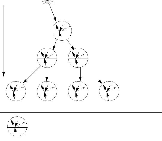
This symbol is used to represent a collision which includes light emitted from the surface, a ray of reflection, and a ray for refraction.
The Basic Concept of Back Tracing Rays
• As seen in Figure above, the light rays may be followed, but the only colors (color explanation follows later) attached to any nodes in this tree are the diffuse lighting from ambient and point sources, and also the specular reflection. After the tree has been fully expanded, the light may be traced forward to the eye. The figure shows the light being propagated back up the tree to the eye (screen pixel).
page 150
Depth = 0
Propagate light |
|
Depth = 1 |
|
||
back through tree |
|
|
Depth = 2
Depth = 3
The Basic Concept of Back Tracing Light Values in a Ray Tree
•This structure gives rise to a tree based on a linked list. Each node in the linked list has:
•Forward and back pointers,
•Surface normals, and optical properties for refraction (used for backtracking),
•The lighting from diffuse and specular sources,
•Vectors for before and after reflection and refraction,
•Positions for ray origins and collision points,
•The depth in the search tree,
•The identification of which object the ray has come from and has hit.
•All of these properties are used in a dynamic fashion, and the list may be grown until all branches have been terminate (i.e. hit background) or are at the maximum search depth.
•This Ray tree structure is constructed with the data stored in a second structure. The second structure for scene data contains geometric information:
•Objects for each ball including centers, radii, and ordered lists of the closest ball,
•An object for the floor, eye, and light, including positions, orientations, and a list of balls, ordered from closest to farthest,
•Transformation matrices,
•The same perspective parameters used in the user interface, •A list of picture areas only filled with background light,