UnEncrypted

J.A. Aledo, S. Martinez, J.C. Valverde

[13]H.S. Mortveit and C.M. Reidys, Discrete, sequential dynamical systems, Discrete Math. 226 (2002) 281–295.

[14]H.S. Mortveit and C.M. Reidys, An Introduction to Sequential Dynamical Systems, Springer, New York, 2007.

[15]Z. Roka´ , Cellular automata on Cayley graphs, Ph.D. Thesis, Ecole Normale Superieure de Lyon, France, 1994.

[16]S. Wiggins, Introduction to Applied Nonlinear Systems and Chaos, Springer, New York, 1990.

[17]S. Wolfram, Statistical mechanics of cellular automata, Rev. Mod. Phys. 55 (3) (1983) 601–644.

[18]S. Wolfram, Universality and Complexity in cellular automata, Physica D 10 (1984) 1–35.

Proceedings of the 12th International Conference on Computational and Mathematical Methods in Science and Engineering, CMMSE 2012 July, 2-5, 2012.

Parallel Dynamical Systems with Di erent Local Functions

Juan A. Aledo1, Silvia Martinez1 and Jose C. Valverde1

1 Department of Mathematics, University of Castilla-La Mancha

emails: JuanAngel.Aledo@uclm.es, Silvia.MSanahuja@uclm.es,

Jose.Valverde@uclm.es

Abstract

In this work, we extend the manner of defining the evolution update of discrete dynamical systems on Boolean functions, without limiting the local functions to be dependent restrictions of a global one. We analyze the cases concerned with parallel dynamical systems (PDS) with the OR, AND, NAND and NOR functions as independent local functions. This extension of the update method widely generalizes the traditional one where only a global Boolean function is considered for establishing the evolution operator of the system. Besides, our analysis allows us to show a richer dynamics in these parallel systems on independent local functions.

Keywords: Discrete dynamical systems; parallel dynamical systems; graphs; Boolean functions.

MSC 2000: 37B99; 37E15; 37N99; 68R10; 94C10.

1Introduction

Computer processes involve generation of dynamics by iterating local mappings. In fact, a computer simulation is a method for the composition of iterated mappings, typically with local dependency regions [5]. It means that the mappings have to be updated in a specific manner, i.e., an update schedule. Update scheduling is also a commonly studied aspect in discrete event simulations [3, 8, 9].

For convenience, it is common to rename the local mappings as entities, which are the lowest level of aggregation of the system. In computer processes, there are many entities

Parallel Dynamical Systems with Different Local Functions

an each entity has a state at a given time (see [5, 6, 7]). The update of the states of the entities constitutes an evolution in time of the system, i.e., a discrete dynamical system (see [4, 11]).

The update of the states is determined by relations of the entities, which are represented by a dependency graph, and local rules, which together constitute the (global) evolution operator of the dynamical system (see [10], [13]). Actually, by means of Boolean functions, local (Boolean) rules to obtain an output from some inputs are obtained. That is, for updating the state of any entity, it is normally considered a Boolean function that acts only on the state of that entity itself and the states of the entities related to it.

If the states of the entities are updated in a parallel manner, the system is called a parallel dynamical system (PDS) [1, 2, 4], while if they are updated in a sequential order, the system is named sequential dynamical system (SDS) [4, 11, 12]. Thus, the evolution or update of a PDS or SDS is usually implemented by local functions which are dependent restrictions of a given global Boolean function.

However, in practice, the rule for the information exchange among one entity and those related to it in the system can be di erent from one entity to another. That is, an entity i can exchange information with the entities related to it by means of a rule fi, while an entity j can do that by means of another rule fj completely independent or di erent from the rule fi.

For this reason, in this work we extend the way of defining the update of discrete dynamical systems on Boolean functions, without limiting the local functions to be dependent restrictions of a global one. This extension of the update method widely generalizes the traditional one, where only a global Boolean function is considered for establishing the evolution operator of the system, and gives as a result a larger variety of discrete dynamical systems on Boolean functions.

We focus on the cases concerned with parallel dynamical systems (PDS) with the OR, AND, NAND and NOR functions as (independent) local functions, determining the orbit structure of this kind of systems. Our analysis allows us to show a richer dynamics in these parallel systems on independent local functions in comparison with the traditional ones (see [1, 4]).

Acknowledgements

This work has been partially supported by the grants MTM2011-23221, PEII11-0132-7661 and PEII09-0184-7802.

J.A. Aledo, S. Martinez, J.C. Valverde

References

[1]J.A. Aledo, S. Martinez, F.L. Pelayo and J.C. Valverde, Parallel Dynamical Systems on Maxterms and Minterms Boolean Functions, Math. Comput. Model. 35 (2012) 666–671.

[2]J.A. Aledo, S. Martinez and J.C. Valverde, Parallel dynamical systems over directed dependency graphs, under review.

[3]A. Bagrodia, K.M. Chandy, W.T. Liao, A unifying framework for distributed simulation, ACM Trans. Modeling Computer Simulation 1 (4) (1991) 348-385.

[4]C.L. Barret, W.Y.C. Chen and M.J. Zheng, Discrete dynamical systems on graphs and Boolean functions, Math. Comput. Simul. 66 (2004), pp. 487–497.

[5]C.L. Barret and C.M. Reidys, Elements of a theory of computer simulation I, Appl. Math. Comput. 98 (1999), pp. 241–259.

[6]C.L. Barret, H.S. Mortveit and C.M. Reidys, Elements of a theory of computer simulation II, Appl. Math. Comput. 107 (2002), pp. 121–136.

[7]C.L. Barret, H.S. Mortveit and C.M. Reidys, Elements of a theory of computer simulation III, Appl. Math. Comput. 122 (2002), pp. 325-340.

[8]D. Je erson. Virtual time. ACM Trans. Programming Languages Systems, 7(3) (1985) 404425.

[9]R. Kumar, V. Garg, Modeling and Control of Logical Discrete Event Systems, Kluwer Academic Publishers, Dordrecht, 1995.

[10]Y.A. Kuznetsov, Elements of Applied Bifurcation Theory, Springer, New York, 2004.

[11]H.S. Mortveit and C.M. Reidys, Discrete, sequential dynamical systems, Discrete Math. 226 (2002), pp. 281-295.

[12]H.S. Mortveit and C.M. Reidys, An Introduction to Sequential Dynamical Systems, Springer, New York, 2007.

[13]S. Wiggins, Introduction to Applied Nonlinear Systems and Chaos, Springer, New York, 1990.

Proceedings of the 12th International Conference on Computational and Mathematical Methods in Science and Engineering, CMMSE 2012 July, 2-5, 2012.

Modeling power performance for master–slave applications

Francisco Almeida1, Vicente Blanco1 and Javier Ruiz1

1 Dept. Estad´ıstica, I.O. y Computaci´on, Universidad de La Laguna

emails: falmeida@ull.es, vblanco@ull.es, javer.ruiz@gmail.com

Abstract

With energy costs now accounting for nearly 30 percent of a data centre’s operating expenses, power consumption has become an important issue when designing and executing a parallel algorithm. This paper analyzes the power consumption of MPI aplications following the master–slave paradigm. The analytical model is derived for this paradigm and is validated over a master–slave matrix–multiplication. This analytical model is parameterized through architectural and algorithmic parameters, and it is capable of predicting the power consumption for a given instance of the problem over a given architecture. We use an external, metered, power distribution unit has been that allows to easily measure the power consumption of computing nodes without the needings of dedicated hardware. .

Key words: Energy–e cient algorithms; Power performance

1Introduction

In recent years power consumption has become a major concern in the operation of largescale datacenters and High Performance Computing facilities. As an example, the 10 most powerful supercomputers on the TOP500 List(www.top500.org) each require up to 12 MW of power for the entire system (computing and cooling facilities). As a result, power-aware computing has been recognized as one of critical research issues in HPC systems.

New processor architectures allow power management through a mechanism called Dynamic Voltage and Frequency Scaling (DVFS) where applications or operating system has the ability to select the frequency and voltage on the fly. Depending on required resources for the application you can select a combination of voltage and frequency, denoted as processors state or p-state. Di erent p-states deal to di erent power consumption, allowing power management by applications [6].

Modeling power performance for master–slave applications

receive ( proc , result [ proc ] ) ;

}

/ Slave P r o c e s s o r / receive ( master , work ) ; compute ( work , result ) ; send ( master , result ) ;

Listing 1: Master–slave paradigm

Power measurement can give us information about the energy consumed by systems, but is not su cient for challenges such as attributing power consumption to virtual machines, predicting how power consumption scales with the number of nodes, and predicting how changes in utilization a ect power consumption [3]. These tasks require accurate models of the relationship between resource usage and power consumption. Models based on architectural parameters has been widely developed [4, 5].

We have developed an instrumentation framework based on metered PDUs (Power Distribution Units), allowing to measure the power consumption of HPC nodes while applications are executed. In a similar way we model application performance (execution time) [7, 8], we propose to model power consumption using architectural parameters (number of cores, cache misses, memory access, network latency and bandwidth) and algorithmic parameters (problem size). The analytical power models obtained can be used by schedulers to save energy when applications are executed on HPC systems.

The rest of this paper is organized as follows: Section 2 introduces master–slave paradigm and Section 3 describes our experimental setup and measurement system. In Section 4 we introduce an analytical power model for the proposed application. We show the obtained models on Section 5. Finally, Section 6 summarizes the paper with some conclusions and future work.

2The Master Slave Paradigm

Under the Master–slave paradigm it is assumed that the work W , of size m, can be divided

p

into a set p of independent tasks work1, ..., workp, of arbitrary sizes m1, ..., mp, i=1 mi = m, that can be processed in parallel by the slave processors 1, ..., p. We abstract the master– slave paradigm by the code in Listing 1

The total amount of work W is assumed to be initially located at the master processor, processor p0. The master, according to an assignment policy, divides W into p tasks and

F. Almeida et al

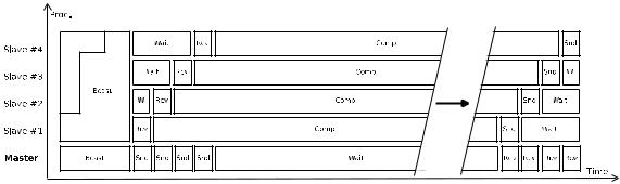
Figure 1: Master-slave diagram of time for matrix multiplication

distributes worki to processor i. After the distribution phase, the master processor collects the results from the processors. Processor i computes worki and returns the solution to the master. The master processor and the p slaves are connected through a network, typically a bus, that can be accessed only in exclusive mode. At a given time-step, at most one processor can communicate with the master, either to receive data from the master or to send solutions back to it. The results are returned back from the slaves as a synchronous round robin.

The transmission time from the master processor to the slave processor i will be denoted by Ri = (βi + τiwi) where wi stands for the size in bytes associated to worki and βi and τi represent the latency and per-word transfer time respectively. This communication cost involves the time for the master to send data to a slave and for it to be received. The latency and transfer time may be di erent on every combination master - slave and they must be calculated separately.

2.1Master–slave matrix–multiplication

We introduce the master–slave matrix–multiplication application as a case study. First of all, we describe de algorithm and the corresponding performance analytical model.

For the master–slave model that we are using in this paper (Fig. 1), the time gets approximately reduced by a factor of 1/p, but a small overload is introduced in the process of broadcasting the matrices and to gather the results. The complete process includes four principal segments: (1) Broadcasting of B matrix, (2) Sending of A matrix by blocks, (3) Waiting for slaves to finish computing and (4) Receiving of matrix C. The total execution time is:

Modeling power performance for master–slave applications

In order to estimate the time used in the broadcast segment, it is necessary to have determined two parameters related to the network: βbcast and τbcast, which represent the latency and the bandwidth of the network while performing broadcasting operations. These parameters can be obtained performing a test in C with MPI in the system used [1]. The number of elements to be sent is the size of the matrix squared.

The send an receive operations performed in the master–slave paradigm can also be

modeled in a similar way. Again, two parameters are needed, βsnd/rcv and τsnd/rcv, obtained with a test referenced in [12]. The first parameter is the latency, but it has a negligible

e ect, because the sub-blocks to be sent are very few. The τ parameter is the bandwidth in node-to-node communication.

Tcomp can be modeled by well-known complexity formula O(N3) for a sequential matrix– multiplication on each processing element. In Section ?? we give more detail about the model for the computation load and the corresponding energy consumed.

This analytical model to predict the running time of master-slave applications has been widely validated. Our goal now is to obtain a similar analytical model for the power consumption of the master–slave matrix–multiplication algorithm. Section 4 describes de model obtained for this implementation on comodity cluster instrumented with a metered PDU.

3Experimental Setup

The measuring system used is one manufactured by the company Schleifenbauer [10]. The equipment consists of a power distribution unit (PDU) with one input and nine outlets, and a master device called Gateway. The Gateway serves as a hub for the available PDUs. Each PDU is connected to the gateway with standard UTP cable and a RS-485 transport layer at 100 Kbit/s. The Gateway is initially configured through the USB or RS-232 port, assigning it a management IP address. As the Gateway has an Ethernet interface that connects to the appropriate network, this address allows us to access the Gateway through any browser to change its settings, to consult the measurements of any PDU connected and to turn on and o the outlets for each PDU. Gathering of data coming from each PDU is provided through various suitable interfaces (Perl API, HTTP, MySQL, etc.) The setup for the measurements includes the following steps:

1. Setting the IP Gateway with one accessible from our network.

F. Almeida et al

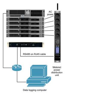
Figure 2: PDU, Gateway and computing nodes connections

2.Mounting the Gateway and the PDU in the data center.

3.Wire UTP cable from the PDU to the Gateway, and back to the PDU, to create a ring in order to provide for additional redundancy.

4.Connect the Gateway to the network.

5.Connect the AC plugs of the nodes of the system under test to the outlets of the PDU. For convenience is advisable to choose consecutive ones.

The equipment installed (Fig. 2) allows the display of consumption data from the PDU by directing a browser to the IP address of the Gateway. The tab “Measurements” allows us to query the data measured in the strip.

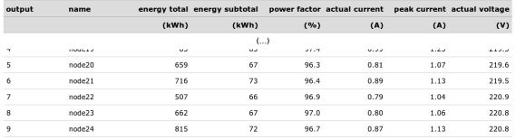
In Fig. 3 that shows the web interface, actual current measurements (RMS) for nodes connected to outlets 5 to 9 can be seen. The values correspond to the actual nodes of the cluster which were used in experimentation. Note that the current at idle is not the same for all nodes, although they are identical models. Also it is worth mentioning that the apparent power is the value of current times voltage, expressed in V · A. The power factor value tell us how much of the apparent energy is converted into usable energy [2]. Values shown are close to 100%, indicating a good design of the power supplies in the compute nodes.

Modeling power performance for master–slave applications

Figure 3: Web interface to the Scheleifenbauer Gateway

RealP ower = VRMS · IRMS · P owerF actor/100

The cluster Tegasaste, used in the experiment, has 24 nodes, five of which connected to the PDU. The front end node is a 4 x Intel(R) Xeon(TM) @ 3.000 GHz with 1 GB RAM. The computation nodes 20 to 24 have 2 x Intel(R) Xeon(TM) @ 3.200 GHz, 1 GB RAM each. The operating system was Linux 2.6.16.16-papi3.2.1 with gcc version 4.3.2 (Debian 4.3.2-1.1) and MPI 1.2.7.For communication between nodes, an Infiniband(R) switch was used.

3.1Measurement

To perform the measurements corresponding to a particular experiment, we use an auxiliary computer, connected to the same network as the Gateway. This auxiliary computer allows the collection of data coming from the PDU, while the algorithm of study is being executed in the parallel cluster, and the logging all the events of interest. The company Schleifenbauer provides an API in Perl to access the measurements. The Gateway has a register type of reading, as current, power factor, voltage, etc.. The user only has to choose the corresponding mnemonic and call the ReadRegisters function. It is important to start this Perl script several seconds before the launching of the execution of the algorithm of study, to take account of the initial values of current in the di erent nodes. Usually a 10 seconds delay was used. Finally another script executes both the Perl script for the PDU and the parallel algorithm in the CPUs.

The execution of this script generates a set of pairs of files, each pair consisting in one file with PDU data and one with CPU data. As already noted, the idle values of current for each node vary, and so the posterior current measurements will be a ected by these idle values. This situation is alleviated by o setting all the measurements, so they are always zero based. The average idle value of current can be added later on to get the real power