

Thermal Analysis of Polymeric Materials
.pdf2.4 Nonequilibrium Thermodynamics |
157 |
__________________________________________________________________
Fig. 2.92
The specific heat capacity at constant pressure can be written as shown in Fig. 2.93, based on the relationship derived in Fig. 2.19. Insertion at constant pressure into Eq. (6) for ds (from Fig. 2.91) leads to the connection to the internal degree of freedom . The first term of the right-hand side of Eq. (16) is the heat capacity of the so-called arrested equilibrium ( = constant). This specific heat capacity is measured when the change in temperature occurs sufficiently fast that the
Fig. 2.93

158 |
|
2 Basics of Thermal Analysis |
__________________________________________________________________ |
||
internal degree of freedom cannot follow ( |
|
|
|
T ) and also if the internal degree of |
|
freedom is frozen ( = 0, because L 0; see Sect. 2.4.6). For the example of the
glass transition, this is the specific heat capacity of the solid, cpo (see Sects. 5.6 and 6.3). In internal equilibrium, one measures the specific heat capacity as expressed in Eq. (18), where ecp is the specific heat-capacity contribution of the internal degree of freedom .
2.4.5 Transport and Relaxation
Time-dependent processes are usually divided into transport phenomena and relaxation phenomena. The transport phenomena cause a move towards equilibrium by transport of, for example, heat, momentum, or mass if there is a difference in the corresponding intensive variables, temperature, pressure, or composition, respectively. Figure 2.94 shows a table of these common transport processes. Naturally there may also be changes of more than one intensive variable at one time. In this case the description of the overall transport processes is more complicated than represented next.
Fig. 2.94
For a transport process to occur, neighboring systems must have different intensive variables. Again, the actual irreversible process is pushed into the boundary between the systems. As an example, the description of heat flow is given in Fig. 2.94. One sets up a hot system, A, next to a colder system, B, both being isolated from the surroundings. The object is to follow the transport of an amount of heat Q in a given time span from A to B, which are closed towards each other. The entropy change in A is Q/Ta, a loss. The entropy change in B is Q/Tb, a gain. The overall change in entropy, S, must, according to the second law, be positive for a

2.4 Nonequilibrium Thermodynamics |
159 |
__________________________________________________________________
spontaneous process, i.e., cause an entropy production. This happens whenever Ta is larger than Tb, as assumed in the figure. Heat flow in the opposite direction would be forbidden by the second law. Note that the absolute magnitude of the heat flux Q is the same in both systems, but the entropies are different.
Relaxation phenomena do not produce any transport, but they do produce a change in an internal degree of freedom, as discussed in Sect. 2.4.4. An internal degree of freedom may be the degree of order of a system. An example of a system with different degrees of order is a carbon monoxide crystal. Two possible structures are C=O C=O C=O C=O, and C=O C=O O=C C=O. Another example of an internal degree of freedom is the surface area of small crystals, discussed in Sects. 2.4.2 and 2.4.3. The thermodynamic description of these internal degrees of freedom is given in Sect. 2.4.4 and the time-dependence is discussed in Sect. 2.4.6.
2.4.6 Relaxation Times
In this section we assume a nonequilibrium process occurs in a homogeneous system. The process is caused by the disturbance of a single internal degree of freedom (see Sect. 2.4.4 for the description of internal degrees of freedom). The independent
variables T(t), p(t), and (t) are directly dependent on time, t. The changes with time, |
||
|
|
|
T dT/dt and p dp/dt, are given by the external perturbation. |
||
|
The change of the internal variable with time, d |
/dt, can be given by a |
dynamic law as shown in Eq. (1) of Fig. 2.95, where a(T,p, |
) is the so-called affinity |
|
which has the meaning of a driving force, and L is the so-called phenomenological coefficient or coupling factor. The first-order kinetics expression, as it is discussed in Chap. 3 for chemical reactions, is shown as Eq. (2) for comparison. The constantis the inverse of the rate constant k and has the dimension of time. It is called the
Fig. 2.95
160 2 Basics of Thermal Analysis
__________________________________________________________________
relaxation time. The concentration is expressed by the number of species N, and Ne corresponds to N at equilibrium, so that (Ne N) is the distance from equilibrium and expresses the driving force. Close to the internal equilibrium, designated by the superscript e, a connection between these two equations can be made. One develops a(T,p, ) into a Taylor series and obtains Eq. (3) of Fig. 2.95. Insertion of Eq. (3) into Eq. (1) yields Eq. (4). By comparison of the coefficients, one can derive an expression for the relaxation time in terms of the thermodynamic functions as given in Eq. (5). This correspondence only applies close to equilibrium, as the derivation reveals. The correspondence is based on the linear term of the Taylor expansion. In actual applications, neither the relaxation-time of Eq. (2) nor (5) need to be constant. This is particularly true if T and p are not kept constant, as indicated.
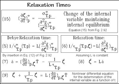
Next, one can make a connection with the discussion of the internal variables of Sect. 2.4.4. Figure 2.96 illustrates the connection between the change of the internal variable with temperature at constant pressure, Eq. (15), and the just derived relaxation time at equilibrium of given T and p, Eq. (5). This relaxation time is also called the Debye relaxation time. Because of the positive curvature at equilibrium drawn in Fig. 2.79, the Debye relaxation time must be 0.
Fig. 2.96
Analogous to the Debye relaxation time, one can introduce the relaxation time of Eq. (6) in Fig. 2.96. This new relaxation time describes also processes further from equilibrium, but it depends on , as indicated. In nonequilibrium T, p, and are
variables that are independent of each other. At constant p one must set (d /dT)p =
T/ . For the change of the affinity with respect to time at constant pressure Eq. (7)
follows from Eqs. (12) and (6). If, furthermore, the coupling factor L is constant, Eqs. (7) and (8) yield at constant pressure the nonlinear differential equation for the determination of the internal variable (t), given as the boxed Eq. (9), where T is the
2.4 Nonequilibrium Thermodynamics |
161 |
__________________________________________________________________
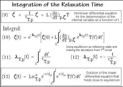
external perturbation of the system. The right side of Eq. (9) expresses also the external force which acts on the internal, molecular degree of freedom. As first integral of Eq. (9) one finds Eq. (10) in Fig. 2.97, with the dimensionless, relative variable of time defined as Eq. (11).
Fig. 2.97
If one assumes the internal equilibrium, e, as the initial state, (0) becomes zero. Furthermore, taking this internal equilibrium as the reference state and assuming that the deviations from Te are small, one can relate all coefficients in Eqs. (9) and (10) to this equilibrium state and consider them to be approximately constant. Equation (10) becomes then a linear differential equation. Its simple integral can be written as Eq. (13). Equation (12) is the easy-to-handle variable of time in terms of the relaxation time.
This description suffices for a first introduction into irreversible thermodynamics. More information is contained in the general references, listed below. In Chap. 3, it will become obvious that the kinetic processes can also be described with detailed, microscopic models of the process. A larger number of applications of the free enthalpy diagrams for crystallization, reorganization, and fusion, discussed in Sect. 2.4.2 will be shown in Chap. 6. The kinetic expressions which can be derived from detailed molecular models, as described in Chap. 3, are used more frequently than the kinetics as it can be derived from the irreversible thermodynamics. One, however, must always be aware that the agreement of a microscopic model with macroscopic experiments is not necessarily proof of the mechanism, while a disagreement is always a reason for either improving or discarding the chosen microscopic model. The just derived kinetic equations based on irreversible thermodynamics are free of any molecular model and are best applied when the linear differential equation holds.

162 2 Basics of Thermal Analysis
__________________________________________________________________
2.5 Phases and Their Transitions
Traditionally a phase is defined in thermodynamic terms as a state of matter that is uniform throughout, not only in chemical composition, but also in physical state. In other words, a phase consists of a homogeneous, macroscopic volume of matter, separated by well-defined surfaces of negligible influence on the phase properties. Domains in a sample, which differ in composition or physical states, are considered different phases. The basic elements of the phases are the atoms and molecules as discussed in Sect. 1.1.3.
A first description will be given of classical (Sects. 2.5.1 and 2.5.5) and mesophases (Sects. 2.5.3 and 2.5.4). It will be shown in Sect. 2.5.2 that sizes of the phases can change from macroscopic (> one m) to microscopic (< one m), to nanophases of only a few nm. Figure 2.98 shows an early suggestion of nanophase structures in polymer fibers [26]. Obviously, one must analyze, to what level such small agglomerations of matter can still function as a phase. When dealing with one component (molecule or part of a molecule of one of the three classes of Chap. 1), one may recognize as many as 57 different phase descriptions [27], based on the constituent molecule, type of phase, and phase size (see Sect. 2.5.2). Finally, an initial insight into phase transitions will be offered in Sects. 2.5.6 and 2.5.7.
Fig. 2.98
2.5.1 Description of Phases
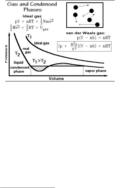
A definitive link between the microscopic and macroscopic description of matter can be given for gases, the most dilute phase as is shown in Figs. 2.8 and 2.9. A schematic representation of a gas frozen in time with indication of the velocity vectors is shown in Fig. 2.99. A graph of the macroscopic, functional relationship
2.5 Phases and Their Transitions |
163 |
__________________________________________________________________
Fig. 2.99
between volume, V, and pressure, p, at constant temperature, T, is also given. The constant R is the universal gas constant (8.3143 J K 1 mol 1). It is rather easy to derive this ideal gas law using the microscopic model of Fig. 2.9. This model of a gas reveals that pV is also equal to (1/3)Nmv2, the right half of the top equation in Fig. 2.5.2. The microscopic parameters are N, m, and v, as listed in Fig. 2.1.9, with the volume, V, having a microscopic as well as macroscopic meaning.
The ideal gas law, as a function of state, does not explain the existence of condensed states of matter, and even for gases, it represents the experimental data only for a dilute gas, i.e., at low p and high T. The basic conditions on which the ideal gas law was derived were: (1) The molecules of an ideal gas should be negligible in volume, (2) have no interactions with the other molecules, and
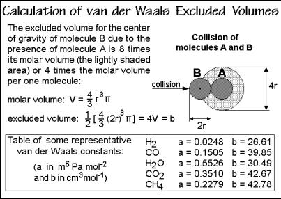
(3) collide elastically. To describe a real gas, the first two conditions must be changed to correspond to the experiment. A simple model which can be used for the description of real gases was proposed by van der Waals1 in 1881. First, he assumed that the molecules, though small, exclude a certain fraction of the total available volume, V, from motion for themselves. At atmospheric pressure, this excluded volume is typically only 0.1%, but at 100 times atmospheric pressure, the excluded volume is as much as 10%. The correction term for the excluded volume, b, is summarized in Fig. 2.100, and expressed with the equation at the top-right in Fig. 2.99. This correction does not change the nature of the gas equation. A simple shift in the volume coordinate by nb leads to the ideal gas curve, similar to the curve shown for the temperature T1.
1 Johannes D. van der Waals, 1837–1923, Professor of Physics at the University of Amsterdam, The Netherlands, received the Nobel Prize in Physics in 1910 for his research on the gaseous and liquid states of matter (van der Waals equation).
164 2 Basics of Thermal Analysis
__________________________________________________________________
Fig. 2.100
The second correction accounts for weak interactions between the molecules. It is done with the constant, a, modifying the measured pressure, p. If one wants to describe a state where molecules are condensed, they must be held together by some interactions which cannot be neglected. Interactions between pairs of molecules are always proportional to the square of concentration, so it is best to give the correction term the form a(n/V)2 and add it to the pressure. The reduction of pressure when molecules attract each other is perhaps obvious if one considers that the molecules that collide with the surface are being attracted away from the surface by the other molecules of the gas. The resulting equation correcting for both the excluded volume and the intermolecular interaction is the van der Waals equation, the boxed equation of Fig. 2.99. The constants, a and b, are different for every gas.
A typical isotherm of a van der Waals equation is drawn in Fig. 2.99 at low temperature T2. At the high temperature T1, the p-V curve is still similar to the ideal gas curve. The effect of the interaction is small (because of the large kinetic energy of the molecules) and nb is small relative to the large V. At T2, one finds a pressure region where three different volumes exist as solution to the van der Waals equation, a first indication that there may be more than just the gaseous state.
If one draws at T2 a horizontal so that the dotted areas above and below the p-V curve are equal, as illustrated in Fig. 2.99, one can show that the two marked states at the ends of the horizontal are equally stable. They are in equilibrium. One can give proof of the stability by using the free enthalpy, discussed in Sect. 2.2. For the moment it is sufficient to know that the two end points are in thermodynamic equilibrium and all intermediate states along the p-V curve are metastable or unstable (they have a higher free enthalpy). The van der Waals equation leads, thus, at certain temperatures and pressures, to the description of two phases in equilibrium, a smallvolume, condensed phase (the liquid), and a large-volume, dilute gas phase (the
2.5 Phases and Their Transitions |
165 |
__________________________________________________________________
vapor). With the introduction of an interaction between the molecules, it is thus possible to understand the connection between liquids and gases. Unfortunately the constants a and b, specific for any one gas, change also with temperature and pressure, limiting the use of the van der Waals equation.
The next step is to use the understanding of the gaseous and liquid states on the microscopic and macroscopic levels to connect to the other condensed states. It is easy to visualize that the liquid is a condensed gas, i.e., neighboring molecules touch frequently, but still move randomly, similar to the gas with all possible forms of large-amplitude motion, summarized in Sect. 2.3.7. Next, one can imagine what happens when the temperature is lowered. The large-amplitude motion must continually decrease and finally stop. As the translational and rotational motion decreases, the liquid becomes macroscopically more viscous. Finally, the large-scale motion becomes practically impossible. Thermal motion continues below this temperature only through vibration. The molecules cannot change their position and the substance becomes solid. In the given case it is an amorphous glass (Gk. !-"#, without form). The structure is the same as that of a liquid, but the changes in position, orientation, and conformational isomeric state of the molecules have stopped. Such a liquid-to-solid transformation occurs at the glass transition temperature, Tg.
To connect liquids to crystals (from Gk. $ , ice), one notes that often molecules are so regular in structure that they order on cooling above the glass transition. In this case, the liquid phase undergoes a more drastic change when solidifying. On crystallization and melting, thus, one finds two changes in the nature of the phase. On crystallization, an ordering occurs, which results in a decrease in entropy, and, helped by the closer packing in the crystal, the large-amplitude motion stops, i.e., a glass transition takes place, as was suggested already in Fig. 1.6.
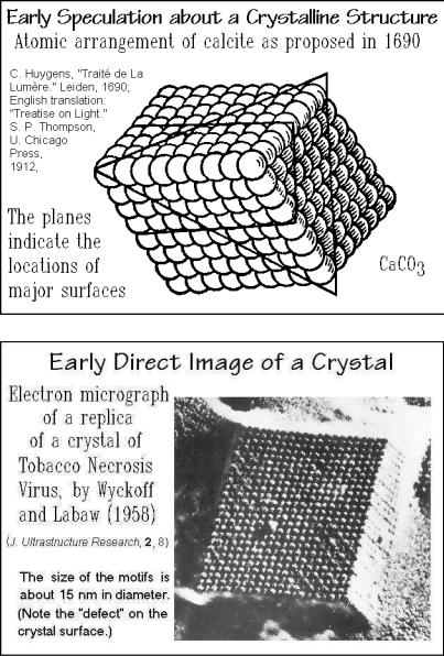
Figure 2.101 illustrates an early picture of the microscopic structure of a crystal, drawn many years before Dalton’s insight into the atomic structure of matter displayed in Chap. 1. At that time there was no knowledge about the shape and size of the molecules. Figure 2.102, in contrast, is a reprint of an early electron micrograph of a crystal with large motifs, where the regular crystalline arrangement can be seen directly. For more detailed description of crystals, see Sect. 5.1.
To round out the discussion of the different states of matter, a schematic summary is given in Fig. 2.103. The four classical phases are listed—gas, melt (liquid), crystal and glass (solids). The main difference between the mobile (fluid) and solid phases are the presence or absence of the three types of large-amplitude motion described in Sect. 2.3.7. In special circumstances, as are addressed in Sect. 2.5.3, not all the largeamplitude motions are frozen. The resulting phase is then intermediate, it is a mesophase (from Gk. , in the middle). The possible mesophases are: Liquid crystals (LC, orientationally ordered and mobile liquids), plastic crystals (PC, positionally ordered crystal with local rotational disorder and mobility), and condis crystals (CD, conformationally disordered and mobile crystals with positional and orientational order). These mesophases are, thus, characterized by an increase of disorder relative to a crystal and by the presence of distinct amounts of largeamplitude molecular motion. On the right-hand side of Fig. 2.103 the possible transitions between these phases are marked and some empirical rules describing the
166 2 Basics of Thermal Analysis
__________________________________________________________________
Fig. 2.101
Fig. 2.102
changes in entropy which are coupled with the disordering are listed. Details about these data are presented in Sect. 5.4. Usually these transitions are first-order transitions (see Sect. 2.5.7). All mesophases, when kept for structural or kinetic reasons from full crystallization on cooling, display in addition a glass transition, as is indicated on the left-hand side of Fig. 2.103. The glass transition leads to a glass