Energy

tegrating along a path, integration along the x -axis in one dimension, as introduced through the work-energy theorem.

Overview: In this chapter, we introduce the concept of energy and energy conservation through two examples: A vertical bowshot and an atom moving along a surface. Based on the examples, we introduce the concept of potential energy for a positiondependent force, a positional energy, to complement the kinetic energy, an energy of motion. For objects subject only to position-dependent force, the sum of the potential and kinetic energy is constant. We can therefore interpret a motion as a transfer of energy between kinetic and potential energies.

We show how to calculate the potential energy for a constant force, a spring force, and a general position-dependent force, and how to use energy conservation to solve mechanics problems. We introduce the energy diagram as an alternative way to analyze and understand motion. We generalize the concept of potential energy to twoand three-dimensional motion. Finally, we introduce the general energy principle, the second law of thermodynamics, and relate external work to changes in the total energy of a system.

11.1 Motivating Examples

The work-energy theorem provides us with an alternative formulation of Newton’s second law that is particularly suited to find the velocity as a function of position in the case when only position-dependent forces act on an object. But we can simplify the analysis even further by the introduction of a position-dependent energy to complement the velocity-dependent kinetic energy, allowing us to use the conservation of total energy as an every quicker way to resolve questions relating the velocity and the position of an object subject only to position-dependent forces. We demonstrate this method by addressing a vertical bowshot and motion along a surface.

Work-Energy as a Conservation Law

How can the work-energy integral be considered a conservation law? And what do we mean by conservation? We know that any motion must satisfy Newton’s second law and its path integral, the work-energy theorem. Let us see how this behaves in a simplified case—for a one dimensional motion with a net force that only depends on the position, F net = F (x ). The work-energy integral is then

where we have introduced the function φ (x ), which is the indefinite integral of F (x ), so that d F/d x = φ (x ). This equation is valid for any two points x0 and x1 along the

motion. We can rearrange this equation, so that all the quantities related to position 0 is on the left hand side and all the quantities related to position 1 is on the right hand side:

The function, K −φ (x ) is a constant along the motion—it is conserved for the motion. We have found an example of a conservation law! Let us examine this conservation law in two simple examples to gain more intuition:

Vertical Shot

If you shoot an arrow vertically upwards, and we neglect air resistance, the arrow is affected by gravity, G = −mg, alone. This is a one-dimensional motion with a net force that only depends on position. (The force is constant and does therefore not depend on anything else than the position). If the arrow starts from y = y0 with a velocity v0, we can apply the work-energy theorem to find the kinetic energy, K1, at any other position, y1. And from the kinetic energy we can find the velocity, v1, if so we please. The work-energy theorem gives:

Let us rearrange this equation so that everything that refers to position 0 is on the left hand side, and everything that relates to position 1 is on the right hand side:

What does this mean? The left hand side is a constant that depends on the initial position, y0, and the initial velocity, v0, of the arrow. But the position y1 on the right hand side can be any position along the motion: This means that the sum mgy + K is constant throughout the motion. How can we interpret the various terms? We have already introduced the notion “kinetic energy” for the velocity-dependent term, K = (1/2)mv2. The mgy term must therefore also have units of energy, and we can interpret this as an energy too. However, this energy does not depend on the velocity of the arrow, but on its position. We call this a positional energy, or more commonly, it is called a potential energy, U = mgy. We see that U is related to the function φ we defined in (11.1). We can now write the work-energy theorem for the motion as:

where we use the term total energy for the term E , which is the sum of the potential and kinetic energies of the arrow.

(2π x /b), and U = F0b/2π , as the potential energy of the atom. We can reorganize the terms, so that all the x0 terms are on the left-hand side:

We notice that the potential energy, U (x ), may be both positive and negative. Hmmm. Is that allowed? Yes. We have not said anything about the signs of the potential energy. Although, the way we have defined kinetic energy does not allow this to become negative. Still, you may be uncomfortable with an initial negative potential energy (although you should get used to this thought by the end of this chapter). There is a simple solution to this: We can add a constant to both sides in (11.10)—and we can add a constant to the function U (x ) since we only care that its derivative dU /d x = −F (x ) and the derivative of a constant will be zero. This means that you are free to determine the zero level of the potential energy. Here, we would like the potential energy to be zero for the initial state, where x = x0, which we achieve with the potential energy:

This is nice and positive for all values of x1 and it is zero at x = 0. Good. Let us use this expression for the potential energy, giving the conservation law:

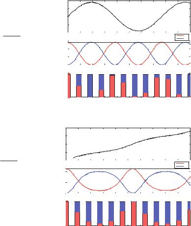
This conservation law gives useful insight into the motion illustrated in Fig. 11.2. The plots show the position x (t ) of the atom for a small initial velocity v0, and corresponding plots of the kinetic, K (t ), and potential, U ′(t ), energies. The atom start with an initial kinetic energy, but no potential energy (we designed the potential energy this way, remember). As it starts moving in the positive x -direction, the potential energy increases, and the kinetic energy decreases, and the atom slows down. Until, at a particular value of x , x = xa , the kinetic energy becomes zero. Since the kinetic energy cannot become less than zero, the atom cannot progress further in the positive x -direction. All the initial kinetic energy is now potential energy. The atom then starts moving in the negative x -direction, increasing its kinetic energy (and therefore speed) until it reaches x = 0. Then the kinetic energy decreases again until