

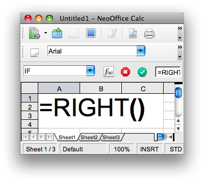
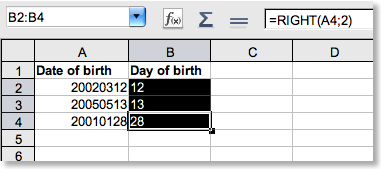
Extracting a given number of characters from a cells, counting from right
Sometimes
you want to extract and use a portion of the contents of a cell,
either number or text.
Just like you can use =LEFT() to
extract characters from the left, you can use =RIGHT() to extract
characters from the right.
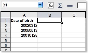 Go
to cell A1 and
enter "Date of birth". Enter these numbers in the cells as
shown.
Go
to cell A1 and
enter "Date of birth". Enter these numbers in the cells as
shown.
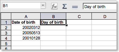 Go
to cell B1 and
enter "Day of birth".
Go
to cell B1 and
enter "Day of birth".
 As
you now can see, the cells A1 and B1 both
act as column headings -- they describe what kind of data you expect
to find below.
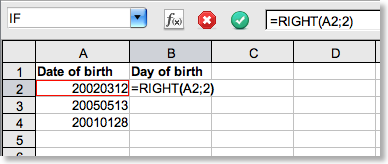
Go to cell B2 and
type =RIGHT(A2;2) and
hit [Enter].
By
the way: instead of typing A2 above,
you can of course use your mouse and click inside cell A2 after
you’ve typed =RIGHT(
As
you now can see, the cells A1 and B1 both
act as column headings -- they describe what kind of data you expect
to find below.
Go to cell B2 and
type =RIGHT(A2;2) and
hit [Enter].
By
the way: instead of typing A2 above,
you can of course use your mouse and click inside cell A2 after
you’ve typed =RIGHT(
 Copy
down the cells from B2 to
the cells B3 and B4.
Do this by selecting cell B2 and
grab the handle in the lower right corner of the cell and drag it
down until you’ve covered B4.
What
happened? Your cell B2 should
now read "12", correct?
Let’s look a bit
closer at what happened here...
What happens is that you
instruct Calc to get the 2 last characters (in this case numbers) in
cell A2 from right.
Copy
down the cells from B2 to
the cells B3 and B4.
Do this by selecting cell B2 and
grab the handle in the lower right corner of the cell and drag it
down until you’ve covered B4.
What
happened? Your cell B2 should
now read "12", correct?
Let’s look a bit
closer at what happened here...
What happens is that you
instruct Calc to get the 2 last characters (in this case numbers) in
cell A2 from right.
=MID()
Extracting a given number characters, counting from the point you specify
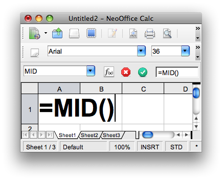
The
formulas =LEFT() and =RIGHT() are
excellent if you want to extract the values from either the first
character from the left or the right side. But what if you want to
extract the value in the middle of a string -- say character 3
through 6 of a total of 14 characters?
It could actually
be done with =LEFT() and =RIGHT() in
conjunction with =LEN(),
but that would be a little complex, esp. as long as we have the
excellent formula =MID(),
which we will show you here.
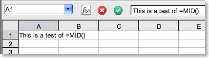 In
cell A1 enter
the following text: [This is a test of
=MID()]
In
cell A1 enter
the following text: [This is a test of
=MID()]
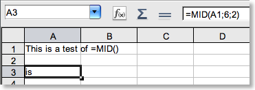
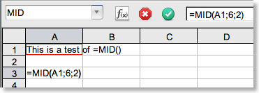 In
cell A3 enter
the following, like shown above: [=MID(A1;6;2)]
What
happens when you press [Enter]?
You get the word [is],
right?
In
cell A3 enter
the following, like shown above: [=MID(A1;6;2)]
What
happens when you press [Enter]?
You get the word [is],
right?
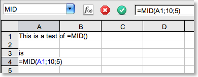 In
cell A4 enter
the following, like shown above: [=MID(A1;10;5)]
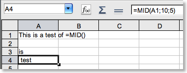
What
happens when you press [Enter]?
You get the word [ test],
right? This illustrates one of the dangers, if you can call it that,
when dealing with text -- it appears to say "test", but it
says " test" -- do you see the difference? There’s an
extra space before the word "test", which to Calc is a
completely different word than " test"!
In
cell A4 enter
the following, like shown above: [=MID(A1;10;5)]
What
happens when you press [Enter]?
You get the word [ test],
right? This illustrates one of the dangers, if you can call it that,
when dealing with text -- it appears to say "test", but it
says " test" -- do you see the difference? There’s an
extra space before the word "test", which to Calc is a
completely different word than " test"!
 OK,
move on to some more explanations regarding the syntax...
Look
at the syntax: [=MID(A1;10;5)]
Doesn’t
this look quite similar to the =LEFT() and =RIGHT() syntaxes?
There
is in fact just one difference, and that is the middle part, which
says from which character you want to start the
extracts.
A1 specifies
that the text you want to extract is contained in the cell A1.
You might just as well have replaced A1 with
the text "This is a test of
=MID()", encapsulated by the "-s
at the beginning and end of the text. This is the same as the first
parameter in the =LEFT()and =RIGHT() syntaxes.
10 specifies
at which character you want to start the extract. This is the
parameter that comes in additions to the two parameters in
the =LEFT() and =RIGHT() syntaxes.
5 specifies
the number of characters you want to extract, which is exactly the
same as the last parameter in
the =LEFT() and=RIGHT() syntaxes.
That’s
it! You can now extract values from a string.
OK,
move on to some more explanations regarding the syntax...
Look
at the syntax: [=MID(A1;10;5)]
Doesn’t
this look quite similar to the =LEFT() and =RIGHT() syntaxes?
There
is in fact just one difference, and that is the middle part, which
says from which character you want to start the
extracts.
A1 specifies
that the text you want to extract is contained in the cell A1.
You might just as well have replaced A1 with
the text "This is a test of
=MID()", encapsulated by the "-s
at the beginning and end of the text. This is the same as the first
parameter in the =LEFT()and =RIGHT() syntaxes.
10 specifies
at which character you want to start the extract. This is the
parameter that comes in additions to the two parameters in
the =LEFT() and =RIGHT() syntaxes.
5 specifies
the number of characters you want to extract, which is exactly the
same as the last parameter in
the =LEFT() and=RIGHT() syntaxes.
That’s
it! You can now extract values from a string.
=RAND()