

Average Joe The second formula
Now,
we could of
course turn the notch up a bit, now that we know how formulas work,
and go to a harder formula -- but we won't. We'll do a similar
formula to =sum(),
which is =average().
This
formula works in exactly the
same manner as =sum() --
it is built the same way, has the same criterions and parameters. The
only difference in these two formulas, is what the outcome is. You
now know that =sum() give
you the sum of any number of, eh, numbers. If you can guess what
the =average() formula
does, please mail
here, and receive a brand
new car as a prize... Yes, it gives you the average of any number of,
eh, numbers!
This is very typical for Calc, in that
similar formulas are also very similar to use. This makes it very
much easier to learn new formulas -- you only have to learn the new
formula name, and use the syntax (= the way that the formula want its
input formated) from the similar formula that you already know.
Why
don't we just use the same figures as last time? Like this:
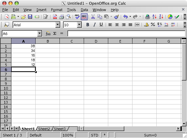 Now,
type =average( and
remember not to
complete the parenthesis:
Now,
type =average( and
remember not to
complete the parenthesis:
 Click
and drag from the cell A1 to
cell A5,
like below:
Click
and drag from the cell A1 to
cell A5,
like below:
 If
you now press [enter] to
finnish the editing of the formula. Pardon? You on the back, speak
up, please! Did I forget to enter the final parenthesis? Hm, yes,
you're right. But did we get an error? Nope, Calc guessed that we had
finished editing the formula and actually completed the
formula for us! If you happened to notice my "error" and
put the end parenthesis yourself, you ended up with exactly the same
result.
If
you now press [enter] to
finnish the editing of the formula. Pardon? You on the back, speak
up, please! Did I forget to enter the final parenthesis? Hm, yes,
you're right. But did we get an error? Nope, Calc guessed that we had
finished editing the formula and actually completed the
formula for us! If you happened to notice my "error" and
put the end parenthesis yourself, you ended up with exactly the same
result.
 Please see
the lesson for =sum() for
further details on the =average() formula,
as they are almost identical in almost every aspect.
Please see
the lesson for =sum() for
further details on the =average() formula,
as they are almost identical in almost every aspect.
The time is now How to let Calc give you time
Sometimes
you want to let Calc give you the current time. You could, of course,
take a look yourself at the watch, but we’re too lazy today, aren’t
we? "Yes we are!". Thanks...
The good news is
that it’s the easiest formula so far. The bad news is that there
aren’t many challenges here -- unless we make them ourselves
:-)
Now, let’s get on with the formula: =NOW()
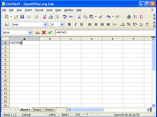 That
is actually the whole, complete formula. Nothing to put between the
parenthesis, nothing. That’s it!
What this formula will
do, is give you the exact date and time, down to the second. But, as
with all other formulas, it won’t recalculate until it’s told to.
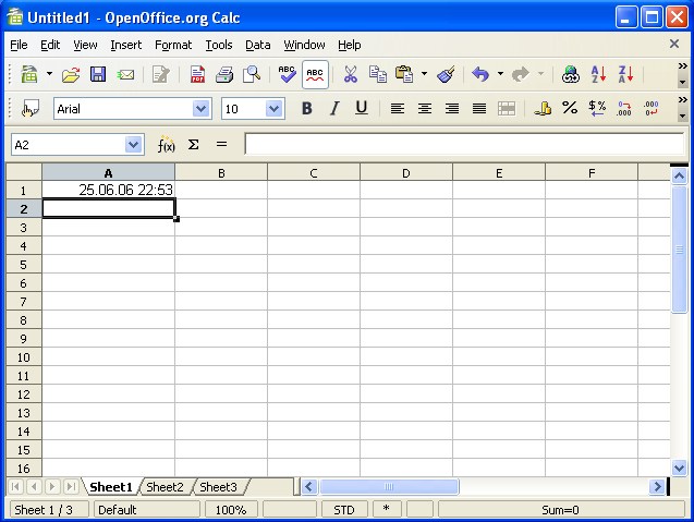
OK, try it now.
Go to any cell, and type =NOW() (it
doesn’t have to be upper case). Calc will now(!) give you the exact
time and date that you pressed [Enter].
If you want it to update the time, double click inside the cell, and
press [Enter]
again. Or you can press [F2]
and hit [Enter].
Or you can go to the Tools ->
Cell Contents menu and
choose Recalculate.
That
is actually the whole, complete formula. Nothing to put between the
parenthesis, nothing. That’s it!
What this formula will
do, is give you the exact date and time, down to the second. But, as
with all other formulas, it won’t recalculate until it’s told to.
OK, try it now.
Go to any cell, and type =NOW() (it
doesn’t have to be upper case). Calc will now(!) give you the exact
time and date that you pressed [Enter].
If you want it to update the time, double click inside the cell, and
press [Enter]
again. Or you can press [F2]
and hit [Enter].
Or you can go to the Tools ->
Cell Contents menu and
choose Recalculate.
=LEFT()
Extracting a given number of characters from a cells, counting from left
Sometimes
you want to extract and use a portion of the contents of a cell,
either number or text.
Let me give you an example. Say you
have entered birth dates in the following format "yyyy-mm-dd",
2004-03-13. It is quite difficult to extract the year of birth here,
especially if you have 13 000 of them...
This is where the
magic of =LEFT() comes
in...
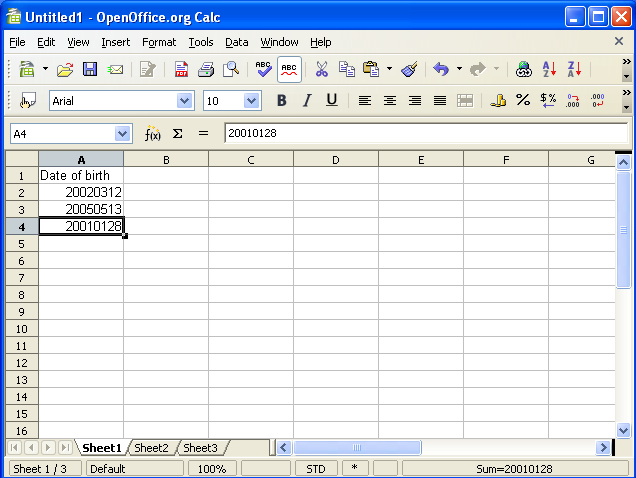
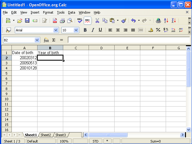
Go to cell A1 and
enter "Date of birth" -- without the "-s. Enter these
numbers in the cells below:
 Go
to cell B1 and
enter "Year of birth".
Go
to cell B1 and
enter "Year of birth".
 As
you now can see, the cells A1 and B1 both
act as column headings -- they describe what kind of data you expect
to find below.
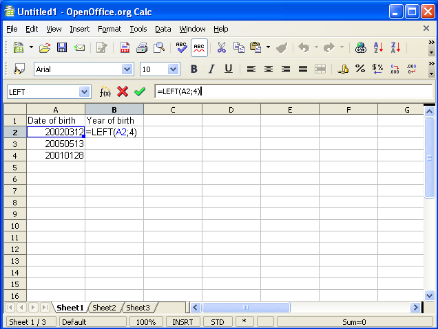
Go to cell B2 and
type =LEFT(A2;4) and
hit [Enter].
By
the way: instead of typing A2 above,
you can of course use your mouse and click inside cell A2 after
you’ve typed =LEFT(
As
you now can see, the cells A1 and B1 both
act as column headings -- they describe what kind of data you expect
to find below.
Go to cell B2 and
type =LEFT(A2;4) and
hit [Enter].
By
the way: instead of typing A2 above,
you can of course use your mouse and click inside cell A2 after
you’ve typed =LEFT(
 Copy
down the cells from B2 to
the cells B3 and B4.
Do this by selecting cell B2 and
grab the handle in the lower right corner of the cell and drag it
down until you’ve covered B4.
Copy
down the cells from B2 to
the cells B3 and B4.
Do this by selecting cell B2 and
grab the handle in the lower right corner of the cell and drag it
down until you’ve covered B4.
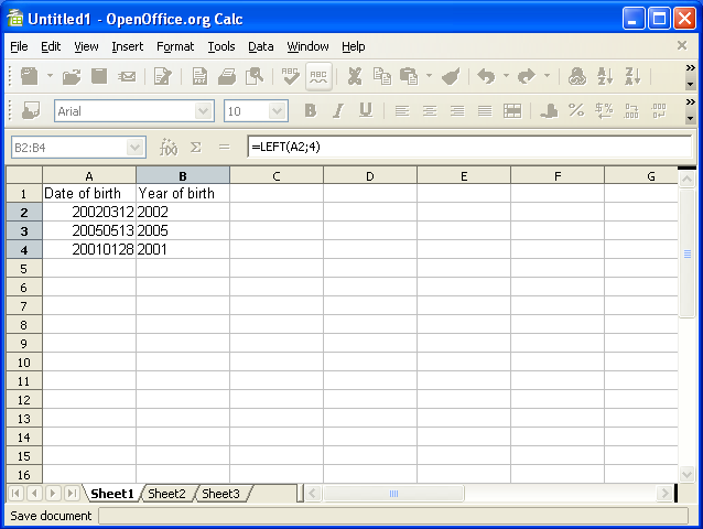 What
happened? Your cell B2 should
now read "2002", correct?
Let’s look a bit
closer at what happened here...
What happens is that you
instruct Calc to
get the 4 first characters (in this case numbers) in cell A2 from
left.
What
happened? Your cell B2 should
now read "2002", correct?
Let’s look a bit
closer at what happened here...
What happens is that you
instruct Calc to
get the 4 first characters (in this case numbers) in cell A2 from
left.
=RIGHT()