p41

INTRODUCTION TO QCD

Michelangelo L. Mangano

CERN, TH Division, Geneva, Switzerland

Abstract

I review in this series of lectures the basics of perturbative quantum chromodynamics and some simple applications to the physics of high-energy collisions.

1.INTRODUCTION

Quantum Chromodynamics (QCD) is the theory of strong interactions. It is formulated in terms of elementary fields (quarks and gluons), whose interactions obey the principles of a relativistic QFT, with a non-abelian gauge invariance SU(3). The emergence of QCD as theory of strong interactions could be reviewed historically, analyzing the various experimental data and the theoretical ideas available in the years 1960–1973 (see e.g. Refs. [17,18]). To do this accurately and usefully would require more time than I have available. I therefore prefer to introduce QCD right away, and to use my time in exploring some of its consequences and applications. I will therefore assume that you all know more or less what QCD is! I assume you know that hadrons are made of quarks, that quarks are spin-1/2, colour-triplet fermions, interacting via the exchange of an octet of spin-1 gluons. I assume you know the concept of running couplings, asymptotic freedom and of confinement. I shall finally assume that you have some familiarity with the fundamental ideas and formalism of QED: Feynman rules, renormalization, gauge invariance.

If you go through lecture series on QCD (e.g., the lectures given in previous years at the CERN Summer School, Refs. [9–11]), you will hardly ever find the same item twice. This is because QCD today covers a huge set of subjects and each of us has his own concept of what to do with QCD and of what are the “fundamental” notions of QCD and its “fundamental” applications. As a result, you will find lecture series centred around non-perturbative applications, (lattice QCD, sum rules, chiral perturbation theory, heavy quark effective theory), around formal properties of the perturbative expansion (asymptotic behaviour, renormalons), techniques to evaluate complex classes of Feynman diagrams, or phenomenological applications of QCD to possibly very different sets of experimental data (structure functions, deep-inelastic scattering (DIS) sum rules, polarized DIS, small x physics (including hard pomerons, diffraction), LEP physics, pp collisions, etc.

I can anticipate that I will not be able to cover or to simply mention all of this. After introducing some basic material, I will focus on some elementary applications of QCD in high-energy e+e , ep and pp collisions. The outline of these lectures is the following:

1.Gauge invariance and Feynman rules for QCD.

2.Renormalization, running coupling, renormalization group invariance.

3.QCD in e+e collisions: from quarks and gluons to hadrons, jets, shape variables.

4.QCD in lepton-hadron collisions: DIS, parton densities, parton evolution.

5.QCD in hadron-hadron collisions: formalism, W=Z production, jet production.

Given the large number of papers which contributed to the development of the field, it is impossible to provide a fair bibliography. I therefore limit my list of references to some excellent books and review articles covering the material presented here, and more. Papers on specific items can be easily found by consulting the standard hep-th and hep-ph preprint archives.

41

2.QCD FEYNMAN RULES

There is no free lunch, so before starting with the applications, we need to spend some time developing the formalism and the necessary theoretical ideas. I will dedicate to this purpose the first two lectures. Today, I concentrate on Feynman rules. I will use an approach which is not canonical, namely it does not follow the standard path of the construction of a gauge invariant Lagrangian and the derivation of Feynman rules from it. I will rather start from QED, and empirically construct the extension to a nonAbelian theory by enforcing the desired symmetries directly on some specific scattering amplitudes. Hopefully, this will lead to a better insight into the relation between gauge invariance and Feynman rules. It will also provide you with a way of easily recalling or checking your rules when books are not around!

2.1.Summary of QED Feynman rules

We start by summarizing the familiar Feynman rules for Quantum Electrodynamics (QED). They are obtained from the Lagrangian:

where is the electron field, of mass m and coupling constant e, and F is the electromagnetic field strength.

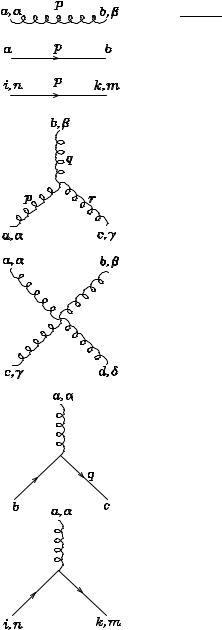
The resulting Feynman rules are summarized in the following table:

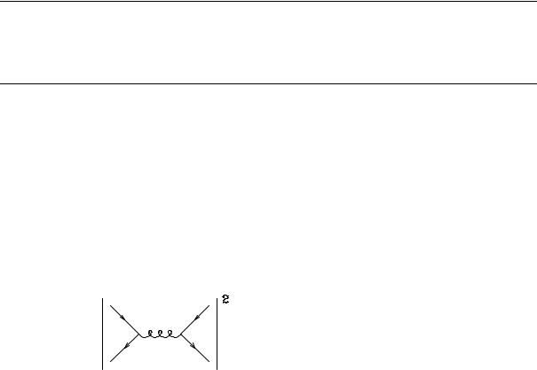
Let us start by considering a simple QED process, e+e ! (for simplicity we shall always assume m = 0):

42

Another way of saying this is that the theory is invariant if (k) ! (k)+ f (k) k . This is the standard Abelian gauge invariance associated to the vector potential transformations:

Notice that the two diagrams are not individually gauge invariant, only the sum is. Notice also that the cancellation takes place independently of the choice of 2. The amplitude is therefore gauge invariant even in the case of emission of non-transverse photons.

Let us try now to generalize our QED example to a theory where the “electrons” carry a nonAbelian charge, i.e., they transform under a non-trivial representation R of a non-Abelian group G (which, for the sake of simplicity, we shall always assume to be of the SU (N ) type. Likewise, we shall refer to the non-abelian charge as “colour”). The standard current operator belongs to the product

the field that couples to the colour current must transform as the adjoint representation of the group G. So the only generalization of the photon field to the case of a non-Abelian symmetry is a set of vector fields transforming under the adjoint of G, and the simplest generalization of the coupling to fermions takes the form:

where the matrices a represent the algebra of the group on the representation R. By definition, they satisfy the algebra:

for a fixed set of structure constants f abc, which uniquely characterize the algebra. We shall call quarks (q) the fermion fields in R and gluons (g) the vector fields which couple to the quark colour current.

with (a; b) colour labels (i.e. group indices) of gluons 1 and 2, (i; j) colour labels of q; q, respectively. Using Eq. (14), we can rewrite (15) as:

43

If we want the charge associated with the group G to be conserved, we still need to demand

The gauge cancellation taking place in QED between the two diagrams is spoiled by the non-Abelian nature of the coupling of quarks to gluons (i.e., a and b do not commute, and f abc 6= 0).

The only possible way to solve this problem is to include additional diagrams. That new interactions should exist is by itself a reasonable fact, since gluons are charged (i.e., they transform under the symmetry group) and might want to interact among themselves. If we rewrite (18) as follows:

we can recognize in the second factor the structure of the qqg vertex. The first factor has the appropriate colour structure to describe a triple-gluon vertex, with a; b; c the colour labels of the three gluons:

Equation (19) therefore suggests the existence of a coupling like (20), with a Lorentz structure V 1 2 3 to be specified, giving rise to the following contribution to qq ! gg:

= i g2 D3 = (ig aij )v(q)i u(q)j

g f abc V ( p; k1; k2) 1 (k1) 2(k2) : (21)

We now need to find V 1 2 3 (p1; p2; p3) and to verify that the contribution of the new diagram to k1 Mg cancels that of the first two diagrams. We will now show that the constraints of Lorentz invariance, Bose symmetry and dimensional analysis uniquely fix V , up to an overall constant factor.

Dimensional analysis fixes the coupling to be linear in the gluon momenta. This is because each vector field carries dimension 1, there are three of them, and the interaction must have total dimension equal to 4. So at most one derivative (i.e. one power of momentum) can appear at the vertex. In priciple, if some mass parameter were available, higher derivatives could be included, with the appropriate powers of the mass parameter appearing in the denominator. This is however not the case. It is important to remark that the absence of interactions with higher number of derivatives is also crucial for the renormalizability of the interaction.

Lorentz invariance requires then that V be built out of terms of the form g 1 2 p 3 . Bose symmetry requires V to be fully antisymmetric under the exchange of any pair ( i; pi) $ ( j ; pj ) since the colour structure f abc is totally antisymmetric. As a result, for example, a term like g 1 2 p3 3 vanishes under antisymmetrization, while g 1 2 p1 3 doesn't. Starting from this last term, we can easily add the pieces required to obtain the full antisymmetry in all three indices. The result is unique, up to an overall factor:

44

To test the gauge variation of the contribution D3, we set 3 = ; 1 = k1 and k3 = (k1 + k2) in Eq. (21), and we get:

The first term cancels the gauge variation of D1 + D2 provided V0 = 1, the second term vanishes for a physical gluon k2, since in this case k2 2 = 0. D1 + D2 + D3 is therefore gauge invariant but, contrary to the case of QED, only for physical external on-shell gluons.

Having introduced a three-gluon coupling, we can induce processes involving only gluons, such as gg ! gg:

(25)

Once more it is necessary to verify the gauge invariance of this amplitude. It turns out that one more diagram is required, induced by a four-gluon vertex. Lorentz invariance, Bose symmetry and dimensional analysis uniquely determine once again the structure of this vertex. The overall factor is fixed by gauge invariance. The resulting Feynman rule for the 4-gluon vertex is given in Fig. 1.

You can verify that the 3- and 4-gluon vertices we introduced above are exactly those which arise from the Yang–Mills Lagrangian:

It can be shown that the 3- and 4-gluon vertices we generated are all is needed to guarantee gauge invariance even for processes more complicated than those studied in the previous simple examples. In other words, no extra 5- or more gluon vertices have to be introduced to achieve the gauge invariance of higher-order amplitudes. At the tree level this is the consequence of dimensional analysis and of the locality of the couplings (no inverse powers of the momenta can appear in the Lagrangian). At the loop level, these conditions are supplemented by the renormalizability of the theory [3,7].

Before one can start calculating cross-sections, a technical subtlety that arises in QCD when squaring the amplitudes and summing over the polarization of external states needs to be discussed. Let us again start from the QED example. Let us focus, for example, on the sum over polarizations of photon k1:

The two independent physical polarizations of a photon with momentum k = (k0; 0; 0; k0 ) are given byL;R = (0; 1; i; 0)=p2. They satisfy the standard normalization properties:

L L = 1 = R R L R = 0 :

45

h i

= gf abc g (p q) + g (q r) + g (r p)

= gf abc q

= ig aki mn

Fig. 1: Feynman rules for QCD. The solid lines represent the femions, the curly lines the gluons, and the dotted lines represent

the ghosts.

46

=L;R

We could have written the sum over physical polarizations using any other momentum ` , provided k ` 6= 0. This would be equivalent to a gauge transformation (prove it as an exercise). In QED the second term in Eq. (28) can be safely dropped, since k M = 0. As a cross check, notice that k M = 0 implies M0 = M3, and therefore:

=L;R

Therefore, the production of the longitudinal and time-like components of the photon cancel each other. This is true regardless of whether additional external photons are physical or not, since the gauge invariance k1 M = 0 shown in Eq. (12) holds regardless of the choice for 2, as already remarked. In particular,

(for n photons, k1 1 k2 2 : : : knn M 1 :::n = 0) and the production of any number of unphysical photons vanishes. The situation in the case of gluon emission is different, since k1 M / 2 k2, which vanishes only for a physical 2. This implies that the production of one physical and one non-physical gluons is equal to 0, but the production of a pair of non-physical gluons is allowed! If 2 k2 6= 0, then M0 is not equal to M3, and Eq. (28) is not equivalent to P = g .

Exercise: show that

In the case of non-Abelian theories, it is therefore important to restrict the sum over polarizations and (because of unitarity) the off-shell propagators to physical degrees of freedom with the choice of physical gauges. Alternatively, one has to undertake a study of the implications of gauge-fixing in non-physical gauges for the quantization of the theory (see Refs. [3,7]). The outcome of this analysis is the appearance of two colour-octet scalar degrees of freedom (called ghosts) whose rˆole is to enforce unitarity in nonphysical gauges. They will appear in internal closed loops, or will be pair-produced in final states. They only couple to gluons. Their Feynman rules are supplemented by the prescription that each closed loop should come with a 1 sign, as if they obeyed Fermi statistics. Being scalars, this prescription breaks the spin-statistics relation, and leads as a result to the possibility that production probabilities be negative. This is precisely what is required to cancel the contributions of non-transverse degrees of freedom appearing in non-physical gauges. Adding the ghosts contribution to qq ! gg decays (using the Feynman rules from Fig. 1) gives in fact

47

The detailed derivation of the need for and properties of ghosts (including their Feynman rules and the “ 1” prescription for loops) can be found in the suggested textbooks. I will not derive these results here since we will not need them for our applications (we will use physical gauges or will consider processes not involving the 3g vertex). The full set of Feynman rules for the QCD Lagrangian is given in Fig. 1.

2.2.Some useful results in colour algebra

The presence of colour factors in the Feynman rules makes it necessary to develop some technology to evaluate the colour coefficients which multiply our Feynman diagrams. To be specific, we shall assume the gauge group is SU (N ). The fundamental relation of the algebra is

with f abc totally antisymmetric. This relation implies that all matrices are traceless. For practical calculations, since we will always sum over initial, final, and intermediate state colours, we will never need the explicit values of f abc. All of the results can be expressed in terms of group invariants (a.k.a. Casimirs), some of which we will now introduce. The first such invariant (TF ) is chosen to fix the normalization of the matrices :

where by convention TF = 1=2 for the fundamental representation. Should you change this convention, you would need to change the definition (i.e. the numerical value) of the coupling constant g, since g a appears in the Lagrangian and in the Feynman rules.

Exercise: Show that tr( a b) is indeed a group invariant. Hint: write the action on a of a general group transformation with infinitesimal parameters b as follows:

b;c

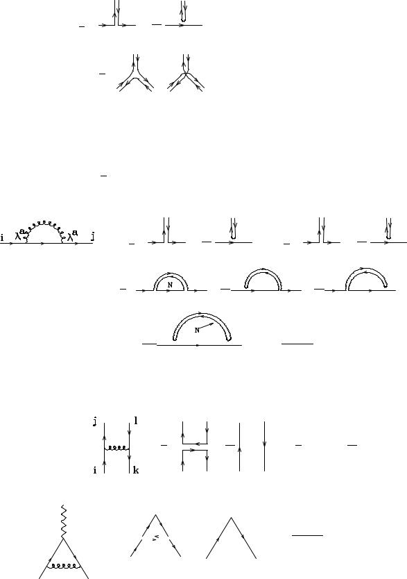
The definition of TF allows to evaluate the colour factor for an interesting diagram, i.e. the quark self-energy:

where we used the fact that ab ab = N 2 1, the number of matrices a (and of gluons) for SU (N ).

There are some useful graphical tricks (which I learned from P. Nason, Ref. [9]) which can be used to evaluate complicated expressions. The starting point is the following representation for the quark and gluon propagators, and for the qqg and ggg interaction vertices:

48

Contraction over colour indices is obtained by connecting the respective colour (or anticolour) lines. A closed loop of a colour line gives rise to a factor N , since the closed loop is equivalent to the trace of the unit matrix. So the above representation of the qqg vertex embodies the idea of “colour conservation”, whereby the colour-anticolour quantum numbers carried by the qq pair are transferred to the gluon. The piece proportional to 1=N in the qqg vertex appears only when the colour of the quark and of the antiquark are the samep. It ensures that a is traceless, as it should. This can be easily checked as an exercise. The factor 1= 2 is related to the chosen normalization of TF .

As a first example of applications, let us reevaluate CF :

C

C

C

C

A

As an exercise, you can calculate the colour factor for qq ! qq scattering, and show that:

This result can be used to evaluate the one-loop colour factors for the interaction vertex with a photon:

49

For the interaction with a gluon we have instead:

Notice that in the case of the coupling to the photon the qq pair is in a colour-singlet state. The gluon exchange effect in this case has a positive sign () attraction). In the case of the coupling to the gluon the qq pair is in a colour-octet state, and the gluon-exchange correction has a negative sign relative to the Born interaction. The force between a qq pair is therefore attractive if the pair is in a colour-singlet, while it is repulsive if it is in a colour-octet state! This gives a qualitative argument for why no colour-octet qq bound state exists.

The remaining important relation that one needs is the following:

a;b

You can easily prove it by using the graphical representation given in Eq. (41), or by using Eq. (43) and f abc = 2i tr([ a; b] c).

3.RENORMALIZATION, OR: “THEORISTS ARE NOT AFRAID OF INFINITIES!”

QCD calculations are extremely demanding. Although perturbative, the size of the coupling constant even at rather large values of the exchanged momentum, Q2, is such that the convergence of the perturbative expansion is slow. Several orders of perturbation theory (PT) are required in order to obtain a good accuracy. The complexity of the calculations grows dramatically with the order of the approximation. As an additional complication, the evaluation of a large class of higher-order diagrams gives rise to results which are a priori ill-defined, namely to infinities. A typical example of what is known as an ultraviolet divergence, appears when considering the corrections to the quark self-energy. Using the Feynman rules presented in the previous lecture, one can obtain:

where simple manipulations lead to the following expression for (p):

50