guide2008_en

BENEFIT TRANSFER – SELECTED REFERENCES FROM INTERNATIONAL LITERATURE

Adamowicz, W., Louviere, J. and Williams, M., 1994. Combining revealed and stated preference methods for valuing environmental amenities. Journal of Environmental Economics and Management 26:271-292.

Alberini, A., Cropper, M., Fu, T.-T., Krupnick, A. Liu, J.-T, Shaw, D. and Harrington W. 1997, Valuing health effect of air pollution in developing countries: the case of Taiwan, Journal of Environmental Economics and Management, 34 (2), 107-26.

Bergstrom, J.C. and De Civita, P., 1999. Status of Benefits Transfer in the United States and Canada: A Review, Canadian Journal of Agricultural Economics 47, pp. 79-87.

Boyle, K. J. and Bergstrom, J. C., 1992. Benefit Transfer Studies: Myths, Pragmatism and Idealism, Water Resources Res. 28(3), pp. 657-663. Brouwer, R. and Bateman, I., 2005, The temporal stability of contingent WTP values, Water Resource Research, 4(3) W03017.

Brouwer, R. and F. A. Spaninks, 1999. The Validity of Environmental Benefit Transfer: Further Empirical Testing, Environmental and Resource Economics, 14, pp. 95-117.

Desvousges, W.H., Johnson, F.R. and Banzhaf, H., 1998. Environmental Policy Analysis with Limited Information: Principles and applications of the transfer method. Massachusetts: Edward Elgar.

Downing, M., Ozuna Jr., T., 1996. Testing the Reliability of the Benefit Function Transfer Approach. Journal of Environmental Economics and Management. 30(3), pp. 316-322.

Garrod, G. and Willis, K., 1999, Benefit Transfer, in Economic Valuation of the Environment: Methods and Case Studies, Edward Elgar Publishing Limited, Cheltenham, UK.

Kirchhoff, S., Colby, B.G. and LaFrance, J.F., 1997, Evaluation the Performance of Benefit Transfer: An Empirical Inquiry, Journal of Environmental Economics and Management, 33, pp. 75-93.

Kristofersson, D. and Navrud, S., 2001. Validity Tests of Benefit Transfer: Are We Performing the Wrong Tests?, Discussion Paper D-13/2001, Department of Economics and Social Sciences, Agricultural University of Norway.

Leon, C.J., Vazquez-Polo, F.J., Guerra, N. and Riera, P., 2002, A Bayesian Model for Benefits Transfer: Application to National Parks in Spain, Applied Economics, 34, pp. 749-757.

Lovett, A.A., Brainard, J.S. and Bateman, I.J., 1997, Improving Benefit Transfer Demand Functions: A GIS Approach, Journal of Environmental Management, 51, pp. 373-389.

Ready, R., Navrud, S., Day, B., Dubourg, R., Machado, F., Mourato, S., Spanninks F. and Vazquez, R., 2004. Benefits Transfer in Europe: Are Values Consistent Across Countries?, Environmental and Resource Economics, Volume 29, Number 1, pp. 67 - 82.

Rosenberger, R., Loomis, S. and John, B., 2001. Benefit Transfer of Outdoor Recreation Use Values: A technical document supporting the Forest Service Strategic Plan, (2000 revision). Gen. Tech. Rep. RMRS-GTR-72. Fort Collins, CO: U.S. Department of Agriculture, Forest Service, Rocky Mountain Research Station.

Silva, P., Pagiola, S., 2003, A Review of Valuation of Environmental Costs and Benefits in World Bank Projects, Environmental Economic Series No.94, Environmental Department, Washington DC, the World Bank.

Climate change

Climate change costs have a high level of complexity due to the fact that they are long-term and global and because risk patterns are very difficult to anticipate. As a result there are difficulties in valuing the damage caused. Therefore, a differentiated approach (looking both at the damage and the avoidance strategy) is necessary. In addition long-term risks should be included.

The climate change or global warming impacts on production and consumption activities are mainly caused by emissions of greenhouse gases carbon dioxide (CO2), nitrous oxide (N2O) and methane (CH4). To a smaller extent, emissions of refrigerants (hydro fluorocarbons) from Mobile Air Conditioners (MAC) also contribute to global warming.

Climate change impacts have a special position in external cost assessment:

-climate change is a global issue, so the impact of emissions is not dependent on the location of the emissions;

-greenhouse gases, especially CO2, have a long lifetime in the atmosphere so that present emissions contribute to impacts in the distant future;

-the long-term impacts of continued emissions of greenhouse gases are especially difficult to predict but potentially catastrophic.

Scientific evidence on the causes and future paths of climate change is becoming increasingly consolidated. In particular, scientists are now able to attach probabilities to the temperature outcomes and impacts on the natural environment associated with different levels of stabilisation of greenhouse gases in the atmosphere.

The proportion of greenhouse gases in the atmosphere is increasing as a result of human activity; the sources are summarised in this figure:

230

ANNEX G

EVALUATION OF PPP PROJECTS

It is possible to define as PPP any project in which the investment (or part thereof) is contributed by the private sector and where there is a regulatory contract between the private and public sectors in terms of risk allocation for the provision of the infrastructure and/or the services. The level of PPP complexity will differ according to the sector, the type of project and country, as a function of the risk mitigation mechanisms and the use of project finance to fund the project. The participation of the private sector in the provision of public assets and services assumes that, whatever the contractual arrangement between the two parties, adequate returns on investment - from a strictly financial perspective - must be allowed to occur.

Definition of PPP

Acknowledging the growing importance of the PPP solution at the Community level, the European Commission is progressively working towards the clarification of the PPP concept, the specification of the policies to be adopted in this domain as well as promoting the dissemination of good practices125.

The 2003 EC Guidelines for successful Public–Private Partnerships126, defines PPP as ‘a partnership between the public sector and the private sector for the purpose of delivering a project or a service traditionally provided by the public sector…By allowing each sector to do what it does best, public services and infrastructure can be provided in the most economically efficient manner’.

The Green Paper on Public-Private Partnerships127 refers to PPPs as ‘forms of cooperation between public authorities and the world of business, which aim to ensure the funding, construction, renovation, management or maintenance of an infrastructure or the provision of a service’. The Green Paper singles out the following elements that normally characterize PPPs:

-the relatively long duration of the relationship, involving cooperation between the public partner and the private partner on different aspects of a planned project;

-the method of funding the project, in part from the private sector, sometimes by means of complex arrangements between the various players. Nonetheless, public funds - in some cases rather substantial - may be added to the private funds;

-the important role of the economic operator, who participates in different stages of the project (design, completion, implementation, funding). The public partner concentrates primarily on defining the objectives to be attained in terms of public interest, quality of services provided and pricing policy, and it takes responsibility for monitoring compliance with these objectives;

-the distribution of risks between the public partner and the private partner, with the risks generally borne by the public sector transferred to the latter. However, a PPP does not necessarily mean that the private partner assumes all the risks, or even the majority of the risks linked to the project. The precise distribution of risk is determined case by case, according to the respective abilities of the parties concerned to assess, control and cope with this risk.

125The main documents reflecting initiatives taken by the EC in this specific domain are: Commission Interpretative Communication on Concessions under Community Law (Official Journal C 121 of 29/04/20009); Guidelines for Successful Public – Private Partnerships; Directives 2004/17/EC and 2004/18/EC of the European Parliament and of the Council Coordinating the Procedures for the Award of Public Contracts; Green Paper on Public-Private Partnerships; Communication from the Commission on Public-Private Partnerships and Community Law on Public Procurement and Concessions (COM (2005) 569 final, issued on 15.11.2005).

126EC, DG Regional Policy, Guidelines for Successful Public–Private Partnerships, 2003.

127EC, Green Paper on Public-Private Partnerships and Community Law on Public Contracts and Concessions (COM (2004) 327 final).

232

adjustments for Competitive Neutrality, Retained Risk and Transferable Risk to achieve the required service delivery outcomes, and is used as a benchmark for assessing the potential value for money of private party bids.

The PSC should:

-be expressed as the Net Present Cost of a projected cash-flow based on the specified government discount rate over the required life of the contract;

-be based on the most recent or efficient form of public sector delivery for similar infrastructure or related services;

-include Competitive Neutrality adjustments so that there is no net financial advantage between public and private sector ownership;

-contain realistic assessments of the value of all material and quantifiable risks that would reasonably be expected to be transferred to the bidders;

-include an assessment of the value of the material risks that are reasonably expected to be retained by the government.

The assessment requires a number of steps:

First of all a raw PSC has to be estimated, which provides a base costing under the public procurement method where the underlying asset or service is owned by the public sector. This includes all capital and operating costs, both direct and indirect, associated with building, owning, maintaining and delivering the service (or underlying asset) over the same period as the term under the Public Private Partnership, and to a defined performance standard as required under the output specification. One of the keys to constructing a PSC is the identification of the Reference Project. The Reference Project is the most likely and efficient form of public sector delivery that could be employed to satisfy all elements of the output specification.

Figure G.1 Public Sector Comparator

Competitive Neutrality adjustments remove any net advantages (or disadvantages) that accrue to a government business simply by virtue of being owned by the government. This allows a fair and equitable assessment between a PSC and the bidders.

Transferable risk Estimate of the value of those risks (from the government’s perspective) that are likely to be allocated to the private party.

Retained risk Estimate of the value of those risks or parts of a risk that the government proposes to bear itself.

Risk adjustment bids may propose different levels of risk transfer. Before the PSC can be compared against the accepted variant bids, the level of risk transfer proposed in each bid should be analysed to reflect the level of risk transfer proposed by the government.

This is achieved by adjusting the relevant bids through the following method:

-where a bid offers a greater level of risk transfer to the private sector than proposed by the government, the adjustment to the bid cost will be negative (reduce the total bid cost); or

234

ANNEX H

RISK ASSESSMENT

In ex-ante project analysis it is necessary to forecast the future value of variables, with an unavoidable degree of uncertainty. Uncertainty arises either because of factors internal to the project (as, for example, the value of time savings, the timing of the completion of the investment etc.) or because of factors external to the project (for example, the future prices of inputs and outputs of the project).

Risk assessment, in the broad sense, requires:

-sensitivity analysis;

-probability distribution of critical variables;

-risk analysis;

-assessment of acceptable levels of risk;

-risk prevention.

Sensitivity analysis

Sensitivity analysis can be helpful in identifying the most critical variables of a specific project. See Chapter 2 for the suggested approach.

Probability distribution of critical variables

Once the critical variables have been identified, then, in order to determine the nature of their uncertainty, probability distributions should be defined for each variable. A distribution describes the likelihood of occurrence of values of a given variable within a range of possible values.

There are two main categories of probability distribution in literature:

-‘Discrete probability distribution’: when only a finite number of values can occur;

-‘Continuous probability distribution’: when any value within the range can occur.

Discrete distributions

If a variable can assume a set of discrete values, each of them associated to a probability, then it is defined as discrete distribution. This kind of distribution may be used when the analyst has enough information about the variable to be studied, to believe that it can assume only some specific values.

Figure H.1 Discrete distribution

0.20

0.15

0.10

0.05

0.00

Continuous distribution

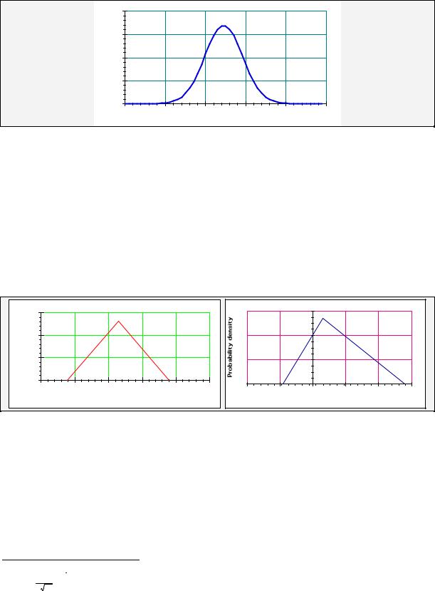
Gaussian (or Normal) distribution is perhaps the most important and the most frequently used probability distribution. This distribution is completely defined by two parameters:

-the mean (μ),

-the standard deviation (σ).

236

Reference Forecasting

The question of where to look for relevant distributions arises. One possible approach is ‘Reference Forecasting’. i.e. taking an ‘outside view’ of the project by placing it in a statistical distribution of outcomes from a class of similar projects. It requires the following three steps:

-the identification of a relevant reference class of past projects, sufficiently broad to be statistically meaningful without becoming too generic;

-the determination of a probability distribution of the outcomes for the selected reference class of project;

-a comparison of the specific project with the reference class distribution and a derivation of the ‘most likely’ outcome.

According to Flyvberg (2005) ‘The comparative advantage of the outside view is most pronounced for non routine projects. It is in planning such new efforts that the biases toward optimism and strategic misrepresentation are likely to be largest.’

Systematic Risk

In financial and economic literature there is a distinction between variability that is random and, at least in principle, diversifiable, and variability that is correlated with overall market trends and economic growth. Non-diversifiable variability is usually described as systematic or market risk.

Risk that is diversifiable, or non-systematic, is regarded for most practical purposes as costless in the public and private sectors. Public sector risks are generally spread across taxpayers, again reducing the variability faced by any individual to a small fraction of individual income.

In welfare economics the cost (or benefit) of systematic variability is conventionally estimated from first principles, using a utility function in which the marginal utility of extra income declines as the individual’s income increases. This can materially affect the estimated value of the benefits of schemes that produce the highest benefits in years when incomes would otherwise have been very low. Such a utility function usually assumes a constant but plausible value for the elasticity of marginal utility with respect to income (normally abbreviated to the ‘elasticity of marginal utility’).

Risk analysis

Having established the probability distributions for the critical variables, it is possible to proceed with the calculation of the probability distribution of the project’s NPV (or the IRR or the BCR). The following table shows a simple calculation procedure that uses a tree development of the independent variables. In the sample reported in the table, given the underlying assumptions, there is 95% probability that the NPV is positive. The more general approach to the calculation of the conditional probability of project performance by the Monte Carlo method was presented in Chapter 2. See also references in the bibliography.

Table H.1 Probability calculation for NPV conditional to the distribution of critical variables (Millions of Euros)

238