

Baumgarten
.pdf144 4 Modeling Spray and Mixture Formation
mass transport into the gas. Due to the enhanced diffusion an increased amount of the energy (transferred from the gas to the liquid) is needed for evaporation, and a quasi-steady state is reached where the droplet temperature stays constant until it is completely vaporized.
It must be pointed out that the use of single-component model fuels is the standard approach today because of its simplicity and low consumption of computational time. Nevertheless, research work today concentrates on more sophisticated evaporation models, especially with respect to modeling more realistic multicomponent fuels and to replace the single-component fuel calculations, see next section.
4.5.2 Evaporation of Multi-Component Droplets
The basic challenge when describing the evaporation process of fuel droplets is the choice of an appropriate reference fuel that represents the relevant behavior of the fuel with sufficient accuracy. For example, in standard CFD simulations, tetradecane (n-C14H30) is normally used to represent the relevant properties of diesel. However, diesel consists of more than 300 different components, and it is obvious that a single reference fuel cannot predict all of the relevant sub-processes during evaporation, ignition, and combustion with sufficient accuracy. Hence, multicomponent model fuels are desirable. The goal is to achieve a high degree of accuracy while keeping the consumption of computational time small.
Initial studies on multi-component fuels concentrated on binary fuels consisting of two discrete hydrocarbons. Both discrete components were implemented in CFD codes using different fuel properties and transport equations for each of the two hydrocarbons. For example, Kneer [65] investigated the evaporation behavior of mixtures consisting of heptane and dodecane as well as hexane and tetradecane. Due to an increased evaporation of the more volatile component, especially during the initial stage of evaporation, these investigations have shown a significantly larger fuel vapor concentration. Further investigations have been published by Jin and Borman [60] and Klingsporn [63], for example. The investigations show that the overall mixture formation process, and thus also ignition and combustion, may be significantly influenced by the composition of the fuel vapor, and that it may be important to describe the multi-component character of fuels more accurately. However, the computational effort describing mixtures of ten and more components is enormous. For example, Rosseel and Sierens [121] developed a model including ten discrete components. According to the authors, the consumption of computational time for simulating the evaporation of a single droplet was twenty times higher than that of a single-component fuel.

4.5 Evaporation |
145 |
|
|
Fig. 4.39. Continuous and discrete representation of multi-component fuels
Tamin and Hallett [137] have shown a possibility of introducing the multicomponent character of fuels without modeling and numerically solving the many differential equations needed to represent a blend of ten or more discrete components. Their approach is based on so-called continuous thermodynamics, which provides a relatively simple and elegant description of mixtures consisting of a multitude of different components. Although the modeling effort is larger compared to a discrete two-component model, the advantage of the continuous thermodynamic approach becomes apparent if more components need to be represented. In this approach, which has been used for gasoline and diesel (e.g. [78, 101, 137, 149, 110]), the composition of the fuel is described by a continuous distribution function.
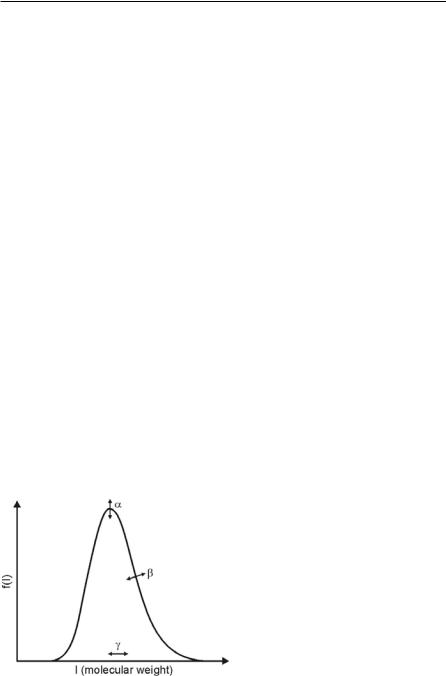
The distribution function characterizes the distribution f(I) of a macroscopic property I of the mixture, for example the molar mass, the boiling temperature, the number of carbon atoms, etc. In the case of hydrocarbon fuels, the molar mass is used as distribution variable. As an example, Fig. 4.39 shows a typical distribution of the different alkanes of diesel and the corresponding continuous distribution function, which has been used to model diesel fuel [77]. The continuous thermodynamic model only needs to solve one set of equations (as in the case of one sin- gle-component fuel) plus two additional equations for the first and the second moment of the distribution function, describing its mean value and variance. The main idea of the continuous thermodynamics approach is the description of the relevant fuel properties needed to determine the evaporation process like boiling and critical temperatures, heat conductivity, heat of evaporation etc. as a function of the distribution variable I. If the distribution of the different components inside the droplet changes during the evaporation process (the more volatile components evaporate first), the distribution function and thus the fuel properties also change. This kind of approach ensures that the effect of the different fuel components on the time-dependent evaporation process is accounted for. It should be mentioned at this point that this condition is only satisfied if the hydrocarbons belong to a particular family of molecules, e.g. alkanes. Hence, it is not possible to model
146 4 Modeling Spray and Mixture Formation
components belonging to different groups, like alkanes and aromatic compounds, with a single distribution function.
Besides the distribution variable, the correct choice of an appropriate mathematical distribution function is necessary. On the one hand, this function must be able to describe the mixture with sufficient accuracy, but on the other hand, the mathematical description should be as simple as possible. In order to describe hydrocarbon mixtures, the so-called gamma-function is used [24, 137, 100]. This distribution function is also known as Pearson type III distribution and is defined as [102]:
|
|
I J |
D 1 |
§ |
|
I J |
|
· |
|
|
|
f (I) |
|
|
|
exp ¨ |
|
¸ |
, |
(4.156) |
|||
|
|
D |
|
|
E |
|
|||||
|
E |
* D |
© |
|
|
¹ |
|
|
|||
|
|
|
|
|
|
||||||
where and Ε and are parameters describing the shape of the curve, and ϑis responsible for the displacement of the origin of the curve, Fig. 4.40.
The quantity I is the distribution variable (molar mass of the fuel components), and ( ) is given by
f |
e ttD 1dt . |
|
* D |
(4.157) |
|
³ |
|
|
0 |
|
|
Because Eq. 4.157 is the normalized gamma-function, the area below the curve is unity:
f |
|
F I ³ f I dI 1 . |
(4.158) |
0 |
|
Thus, the first and the second moment of the distribution are given by
Fig. 4.40. Gamma-function: effect of parameters , Ε, ϑ
|
|
4.5 Evaporation 147 |
|
|
|
|
f |
|
T |
³ f I I dI |
(4.159) |
|
0 |
|
and by |
|
|
|
f |
|
\ |
³ f I I 2 dI . |
(4.160) |
|
0 |
|
The first moment Τ is the mean of the distribution function, and is a measure for the variance ς. In the case of the gamma-function, Τ and can be expressed as
T |
D E J , |
(4.161) |
V 2 |
D E2 , |
(4.162) |
\ |
T2 V 2 . |
(4.163) |
The parameters , Ε, and ϑare chosen in order to achieve the best representation of the specific fuel of interest. The continuous thermodynamics can also be applied to single-component fuels by using extremely narrow distributions. Table 4.4 summarizes the distribution parameters for various fuels as given in the works of Lippert [77] and Pagel [100].
Besides a transport equation for the overall fuel mass fraction, two additional transport equations for the first and the second moment, describing the shape of the distribution function for the vaporized fuel, are necessary in order to determine the change of the vapor phase composition in the computational cell around the evaporating droplet. The relevant vapor phase transport equations have been derived by Tamin and Hallett [137]. For a single component k of the multi-
component fuel the mass transport equation can be written as |
|
|
|
|
||||||||
|
w |
& |
UDk ,av Yk |
d |
C |
|
d |
|
S |
|
|
|
|
|
UYk UuYk |
|
UYk |
|
|
|
UYk |
|
, |
(4.164) |
|
|
wt |
dt |
dt |
|
||||||||
where Yk is the mass fraction of the component k, and Dk,av is the averaged binary diffusion coefficient. The resulting equations are derived by integrating the spe-
cies transport equation over the complete distribution function in order to obtain
Table 4.4. Distribution parameters for multi-component and single-component fuels
|
Diesel |
Gasoline |
n-Octane |
n-Decane |
|
18.5 |
5.7 |
100 |
100 |
Ε |
10 |
15 |
0.1 |
0.1 |
ϑ |
0 |
0 |
104.2 |
132.3 |
Τ |
185 |
85.5 |
114.2 |
142.3 |
ς |
43 |
35.8 |
1 |
1 |

148 4 Modeling Spray and Mixture Formation
the transport equation for the species mass fraction, and by weighting the equation by I and by I2 before integrating in order to get the transport equations for the first and the second moment [78, 137, 46]:
|
|
|
|
w |
& |
|
|
|
|
S |
|
|
C |
|
|
|
|
|
|
|
|
|
|
|
|
|
|
||||
|
|
|
|
|
UYf UuYf |
|
UD Yf UYf |
UYf , |
|
(4.165) |
|||||
|
|
|
|
wt |
|
||||||||||
|
|
|
|
|
|
|
|
|
|
|
|
|
|
|
|
|
w |
|
|
& |
|
UD Yf T UYf T |
S |
C |
|
||||||
|
|
|
UYf T UuYf T |
|
|
|
UYf T |
, |
(4.166) |
||||||
|
wt |
|
|
|
|||||||||||
w |
|
|
|
|
ˆ |
|
|
S |
|
C |
|
||||
wt |
UYf\ UuiYf \ |
|
UD Yf\ UYf\ |
|
|
UYf\ . |
(4.167) |
||||||||
The quantity Yf is the overall fuel mass fraction in the gas, Υ is the mass-averaged |
||||
|
|
|
ˆ |
|
|
|
|||
density, and D,D and |
D are binary diffusion coefficients for the respective con- |
|||
|
|
|
|
ˆ |
served scalars. It can be shown that D | D | D . The first term on the right hand |
||||
side of Eqs. 4.165–4.167 is due to mass diffusion, while the second and the third ones are source terms due to spray evaporation and combustion.
The source term due to spray evaporation is determined by the evaporation of the multi-component fuel droplets. If the droplet interior is assumed to be well mixed, which is usually done in most of the 3D CFD calculations, the molar flux
over the droplet surface is given by |
|
|
|
|
||
|
|
1 |
|
d clVdrop |
, |
(4.168) |
A |
|
dt |
||||
n |
|
|
||||
|
|
drop |
|
|
|
|
where Adrop = 4ΣR2, Vdrop = (4/3)ΣR3, and cl = Υl /Τl is the liquid molar density in mol/cm3. In contrast to the fuel vapor distribution function, the relevant parame-
ters of the liquid fuel distribution inside the droplet are denoted by the subscript l. It should also be mentioned that all liquid-phase composition calculations are performed on a molar basis, since the vapor-liquid equilibrium is solved in a molar frame of reference. Using the expressions for drop surface area and volume in Eq. 4.168, the time-dependent change of droplet radius becomes
dR |
|
R §c dTl |
d Ul · |
n . |
(4.169) |
||||||
|
|
|
¨ |
|
|
|
|
¸ |
|
|
|
|
|
|
l |
|
|
|
|
|
|
||
dt |
|
dt |
|
dt |
cl |
|
|||||
|
3clTl © |
|
|
¹ |
|
||||||
The mole flux n, which is needed to determine the mean and the second moment of the droplet composition, can be calculated equating the fluxes at the liquid/gas interface. In the case of a single component k of the liquid phase, Eq. 4.168 yields
|
|
1 |
|
d xk clVdrop |
|
R |
|
dxk |
, |
(4.170) |
A |
|
dt |
|
|
||||||
nk |
|
xk n cl 3 dt |
|
|||||||
|
|
drop |
|
|
|
|
|
|
|
|

4.5 Evaporation |
149 |
|
|
where xk is the mole fraction of component k in the liquid phase. Because a wellmixed droplet interior is assumed, it is also the mole fraction inside the whole droplet. The mole flux yf,R in the gas phase at the liquid-vapor interface (index R) is given by assuming equal molar diffusion from droplet to gas,
|
|
|
|
dyk |
|
. |
|
|
|
(4.171) |
|
nk |
n yk ,R c Dk ,av |
dr |
|
|
|
||||||
Equating Eq. 4.170 and Eq. 4.171 gives |
|
|
|
R |
|
|
|||||
|
|
|
|
|
|||||||
|
|
|
|
|
|
|
|
|
|||
n xk yk ,R |
c Dk ,av |
dyk |
cl |
|
R dxk |
. |
(4.172) |
||||
|
|
|
|
|
|
|
|
|
|
|
|
|
|
dr |
|
|
|
3 dt |
|
|
|||
|
|
|
|
|
|
|
|
||||
The resulting equations for the liquid composition are derived by integrating over the complete distribution function and by several further transformations [137]:
dTl
dt
d\l
dt
|
|
|
|
|
|
dy f |
|
|
|
|
||
|
|
|
|
|
|
|
|
|
||||
|
n 1 y f ,R |
c D |
|
|
, |
|
|
|||||
dr |
|
|
||||||||||
|
|
|
|
|
|
|
|
|
|
|
||
3 |
ª |
|
|
|
|
|
d |
|
|
º |
|
|
|
|
«n Tl y f T c D |
|
y f T » |
, |
|||||||
|
cl R ¬ |
|
|
|
|
|
dr |
|
|
¼R |
|
|
|
|
|
|
|
|
|
|
|
||||
3 |
ª |
|
|
|
|
ˆ |
d |
|
|
º |
|
|
|
|
«n \l y f \ c D |
|
|
|
y f \ » . |
||||||
cl R |
¬ |
|
|
|
|
|
dr |
¼R |
||||
|
|
|
|
|
||||||||
(4.173)
(4.174)
(4.175)
The index R denotes the droplet surface. Next, equilibrium is assumed at the interface, resulting in
|
|
|
|
y |
f |
r |
|
1 1 y |
|
1 B |
R / r |
|
|
(4.176) |
|||||||
|
|
|
|
|
|
|
|
|
|
|
|
f ,f |
|
|
|
|
|
|
|||
and |
|
|
|
|
|
|
|
|
|
|
|
|
|
|
|
|
|
|
|
|
|
|
|
|
|
|
|
|
1 |
|
|
|
f |
ª |
|
|
|
|
R / r |
º |
|
|
|
I |
|
r |
|
I |
R |
|
|
R |
I |
¬ |
|
B |
|
¼ |
, |
(4.177) |
|||||
B |
|||||||||||||||||||||
|
|
|
|
|
I |
|
|
|
1 |
B 1 |
|
1 |
|||||||||
where Ι represents yΤ and y , respectively. The subscripts “R” and “φ” indicate the gas phase properties at the droplet surface and in the undisturbed surroundings, respectively. B is the Spalding transfer number,
B |
y f ,R y f ,f |
. |
(4.178) |
||
1 |
y f ,R |
||||
|
|
|
|||
Using Eqs. 4.176 and 4.177 in Eqs. 4.174 and 4.175 results in expressions that are only dependent on quantities calculated by assuming equilibrium conditions at the liquid-gas interface (R) and on those of the surrounding (φ). The final expressions describing the change of the mean and the second moment of the droplet composition are

150 4 Modeling Spray and Mixture Formation
dTl
dt
d\l
dt
3n ª
cl R «¬ Tl y f ,R
3n ª
cl R «¬ \l y f ,R
TR B1 Tf y f ,f
\R B1 \f y f ,f
TR y f ,R ȼ , |
(4.179) |
¼ |
|
\R y f ,R ȼ . |
(4.180) |
¼ |
|
The time-dependent development of droplet temperature can be calculated by an energy balance in analogy to Eq. 4.139 as
dTl |
|
3 |
ª |
|
|
º |
, |
(4.181) |
|
||||||||
dt |
|
c c R ¬qconv nhfg ¼ |
||||||
|
|
l v |
|
|
|
|
|
|
where h fg and c v = cv·Τ are the molar heat of evaporation and the molar specific heat of the liquid. The convective heat flux and the molar flux may be approximated by
|
O T |
T |
|
ln 1 B |
|
|
|
|||||
|
f |
l |
|
|
Nu |
(4.182) |
||||||
qconv |
|
2R |
|
|
|
B |
|
|
||||
|
|
|
|
|
|
|
|
|||||
and |
|
|
|
|
|
|
|
|
|
|
|
|
|
|
|
|
|
|
|
|
|
|
|||
n |
|
cD |
|
ln 1 B |
|
Sh . |
|
|
(4.183) |
|||
|
2R |
|
|
|||||||||
|
|
|
|
|
|
|
|
|
||||
The appropriate Nusselt and Sherwood numbers including corrections for the influence of a relative velocity between droplet and gas are
Nu |
2.0 0.6 Re1/ 2 Pr1/ 3 and |
(4.184) |
Sh |
2.0 0.6 Re1/ 2 Sc1/ 3 , |
(4.185) |
where Pr and Sc are the Prandtl and the Schmidt numbers, respectively.
As already mentioned, phase equilibrium is assumed to determine the vapor mole fraction in the gas phase at the droplet’s surface, and Raoult’s law is applied. In the case of a single component, this relation between the mole fraction of vaporized fuel yk at the interface and the mole fraction xk inside the liquid drop is
y |
|
x |
§ |
pk |
· |
, |
(4.186) |
k |
|
¸ |
|||||
|
k ¨ |
p |
|
|
|||
|
|
|
© |
¹ |
|
|
|
where p is the static pressure in the gas phase and pk is the partial pressure of the component k with molar mass I. In the case of a continuous distribution function, the mole fractions of the different components inside the liquid are described by a distribution function, which changes its shape during evaporation. Thus, the mole fractions at the surface also change, and in this case Raoult’s law is derived by integrating over the complete distribution function:
4.5 Evaporation |
151 |
|
|
Fig. 4.41. Boiling temperature of alkanes as function of molecular weight
|
f |
§ p |
k |
I |
|
· |
|
|
y f |
³ |
fl I ¨ |
|
|
¸dI . |
(4.187) |
||
|
p |
|
|
|||||
|
0 |
© |
|
|
|
¹ |
|
|
The value of pk at the interface is given by the Clausius-Clapeyron equation,
pk I |
ªs fg |
§ |
Tb I ·º |
|
|
|||||
p0 exp « |
|
|
|
¨1 |
|
¸» |
, |
(4.188) |
||
|
|
|
Tl |
|||||||
R |
||||||||||
|
« |
© |
¹» |
|
|
|||||
|
¬ |
|
|
|
|
|
¼ |
|
|
|
where p0 = 101.325 kPa is a reference pressure, Tb(I) is the corresponding boiling temperature of component I, s fg is the molar entropy of evaporation in J/(mol·K),
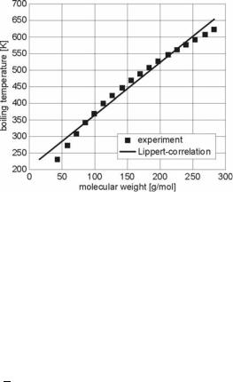
R = 8.314151 J/(mol·K) is the molar gas constant, and Tl is the temperature of the liquid drop. Fig. 4.41 shows the boiling temperature of alkanes as a function of molar mass I. A linear correlation as proposed by Lippert [77] can be assumed,
Tb I ab bb I , |
(4.189) |
where ab and bb are constants obtained from regression of boiling point data. In the case of diesel fuel, Lippert [77] uses ab = 208.53 K and bb = 1.5673 K/mol.
Further quantities needed to calculate the multi-component fuel evaporation process using the continuous thermodynamics approach are the heat of evaporation, the heat conductivity of the gas mixture, the specific heat capacities of gas mixture and liquid, the binary diffusion coefficient between air and fuel vapor, and the critical temperature. It should be noted that for all correlations used to describe the boundary layer the 1/3rd rule of Hubbard et al. [54] is used in order to account for the strong gradients of the quantities of interest and to calculate representative
reference values inside the boundary layer. For example, Tref and Yf,ref are calculated as

152 4 Modeling Spray and Mixture Formation
T |
|
2 |
T |
|
1 |
T , |
|||
|
|
|
|
|
|||||
ref |
|
3 R |
|
3 f |
|||||
and |
|
|
|
|
|
|
|
|
|
Yf ,ref |
2 |
Yf ,R |
1 |
Yf ,f . |
|||||
3 |
|
||||||||
|
|
|
|
3 |
|
||||
(4.190)
(4.191)
The heat of evaporation can be described via an empirical relation. It is assumed that ideal gas behavior can be applied and that pressure effects can be neglected. According to Reid et al. [113] the heat of evaporation for a single component is given as
|
|
|
|
ªlog pcrit 1.013 |
ºª Tcrit T º |
0.38 |
|
||||
|
|
|
|
|
|
||||||
hfg 1.093 |
R Tb « |
|
»« |
|
|
» |
, |
(4.192) |
|||
0.930 T / T |
T |
T |
|||||||||
|
|
¬ |
b crit |
¼ |
|
b ¼ |
|
|
|||
|
|
« |
»¬ crit |
|
|
||||||
where pcrit is the critical pressure and Tcrit is the critical temperature. Tamin and Hallett [137] have modified this approach for multi-component fuel mixtures:
|
|
ª |
ª |
|
1 |
|
|
|
|
ºº |
ª |
Tcrit Tl 0.38 º |
|
|
|
|
|
|
|
|
|
||||||||
hfg «ah bh « y f T |
|
|
ª y f T |
y f T |
º |
»» |
« |
|
» , |
(4.193) |
||||
|
6.959 |
|||||||||||||
¬ |
¬ |
R |
B ¬ |
f |
|
R ¼ |
¼¼ |
« |
» |
|
||||
|
|
|
|
|
|
|
|
|
|
|
¬ |
|
¼ |
|
where ah = 2.07·10-7 and bh = 1.35·10-5 for units of h fg of J/kmol.
The thermal conductivity of a gaseous fuel component can be described as a
function of temperature and molecular weight [137], |
|
O I ,T aKC aKT T bKC bKT T I , |
(4.194) |
where Ο(I, T) is in W/(m·K), aKC = -2.37·10-2, bKT = -1.91·10-8.
A correlation for the specific heat capacity of by Chou and Prausnitz [22]:
aKT = 1.09·10-4, bKC = 3.47·10-5,
the fuel vapor has been developed
cp I ,T |
|
|
acp bcp I , |
|
|
|
||||
R |
|
|
|
|||||||
a |
a |
a |
T a |
T 2 a T 3 |
, |
(4.195) |
||||
cp |
c0 |
|
|
c1 |
c2 |
c3 |
|
|
|
|
b |
b |
b T b T 2 b T 3 |
, |
|
|
|||||
cp |
c0 |
|
c1 |
|
c2 |
c3 |
|
|
|
|
where cp(I, T) is in J/(mol·K), ac0 = 2.465, ac1 = -1.144·10-2, ac2 = 1,759·10-5, |
|
ac3 |
= -5.972·10-9, bc0 = 2.465, bc1 = -1-144·10-2, bc2 = 1.759·10-5, and |
bc3 |
= -5.972·10-9 [77]. |
|
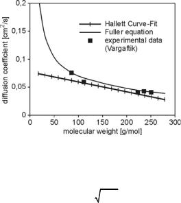
Tamin and Hallett [137] have given a correlation for the binary diffusion coef- |
ficient between alkanes and air. This correlation assumes a linear relation between molar mass and diffusion coefficient. However, for low and very large molar masses, this function underpredicts the diffusivity, see Fig. 4.42. Fuller (see [113]) uses a non-linear approach,
4.5 Evaporation |
153 |
|
|
Fig. 4.42. Binary diffusion coefficients for alkanes and air [77]
Daf |
|
|
|
0.00143 T1.75 |
, |
|||||
p Maf |
ª ¦Q |
1/ 3 |
¦Q 1/ 3 º2 |
|||||||
|
|
|
|
« |
|
|
|
a |
f » |
|
|
|
|
|
¬ |
|
|
|
|
¼ |
(4.196) |
|
|
|
|
|
|
|
|
1 |
|
|
|
|
§ |
1 |
1 · |
|
|
||||
Maf |
2 |
¨ |
|
|
|
|
¸ |
, |
|
|
MW |
T |
f |
|
|
||||||
|
|
© |
a |
|
|
¹ |
|
|
|
|
where T, p, and MWa are the temperature, the pressure and the molecular weight of the surrounding gas, Τf is the mean of the fuel vapor distribution, and 6Θ is the sum of the atomic diffusion volumes of air and fuel [113]. This method shows a much better representation of data from Vargaftik, Fig. 4.42, and it also includes the reciprocal dependency on pressure as predicted by the kinetic theory of gases [77]. Daf is used as binary diffusion coefficient in Eqs. 4.165–4.167.
A linear relation for the critical temperature as function of molecular weight is given by Tamin and Hallett [137],
Tcrit I ac bc I , |
(4.197) |
where ac = 440.8 and bc = 1.21. Lippert [77] modified this approach introducing the critical volume Vcrit,
T |
³Vcrit I Tcrit I f I dI |
. |
(4.198) |
|
|||
crit |
³Vcrit I f I dI |
|
|
|
|
||
The critical volume can be described by a linear function with parameters from Li et al. [75]:
Vcrit I av bv I , |
(4.199) |