

11 ALGEBRA
.pdf
|
17 |
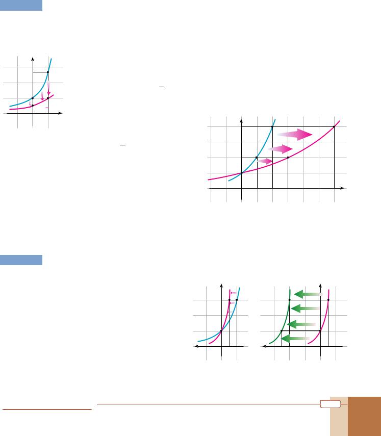
Sketch the graph of y = 3x+2 – 2 and determine its domain, range and asymptote. |
EXAMPLE |
||
|
|
|
Solution |
We will begin with the graph y = 3x. Remember that when more than one transformation is |
|
|
|
applied to a function, we begin the graphical transformation by first considering the changes |
|
|
to the variable. |
|
|
To obtain 3x+2 in terms of f(x) = 3x, we can write g(x) = 3x+2= f(x + 2). So we shift the graph |
|
|
of f(x) = 3x two units to the left (p = 2). Then y = 3x+2 – 2 = g(x) – 2, so we shift the graph |
|
|
of g(x) two units downward (k = 2). |
(–1, 3) |
3 |
(1, 3) |
||
g(x)=3x+2 |
|
|||
|
|
|||
|
|
|
|
|
|
|
2 |
|
|
(–2, 1) |
|
(0, 1) |
|
|
|
|
|
||
|
|
f(x)=3x |
|
|
-2 |
-1 |
0 |
1 |
x |
|
|
-1 |
|
|
|
|
y |
|
|
|
|
|
y |
|
|
(–1, 3) |
|
3 |
|
|
|
|
|
|
|
g(x)=3x+2 |
|
2 |
|
|
|
|
|
|
|
(–2, 1) |
y=3x+2– 2 |
||
|
|
1 |
|
|
|
|
(–1, 1) |
|
|
x |
-2 |
|
0 |
|
|
(–2, –1) |
-1 |
|
|
|
|
|
||
|
|
|
-2 |
y=-2 |
As a result, we can see that y = 3x+2 – 2 has domain , range (–2, ) and asymptote y = –2.
|
|
|
|
|
|
y |
|
EXAMPLE |
18 |
Sketch the graph of y = –2 |
x |
and determine its domain, range |
|
2 |
(1, 2) |
|
|
|
|
||||
|
|
and asymptote. |
|
|
f(x)=2x |
1 |
|
|
|
|
|
|
|
||
|
|
|
|
|
|
|
|
Solution |
We first draw the graph of f(x) = 2x. By reflecting it in the x-axis |
|
0 |
1 |
|||
|
|
we obtain the graph of y = –2x = –f(x). So y = –2x has |
y=-2x |
|
x |
||
|
|
domain , range (– , 0) and asymptote y = 0. |
-1 |
|
|||
|
|
|
|
||||
|
|
|
|
|
|
-2 (1, -2) |
|
Exponential and Logarithmic Functions |
|
|
|
|
129 |
||

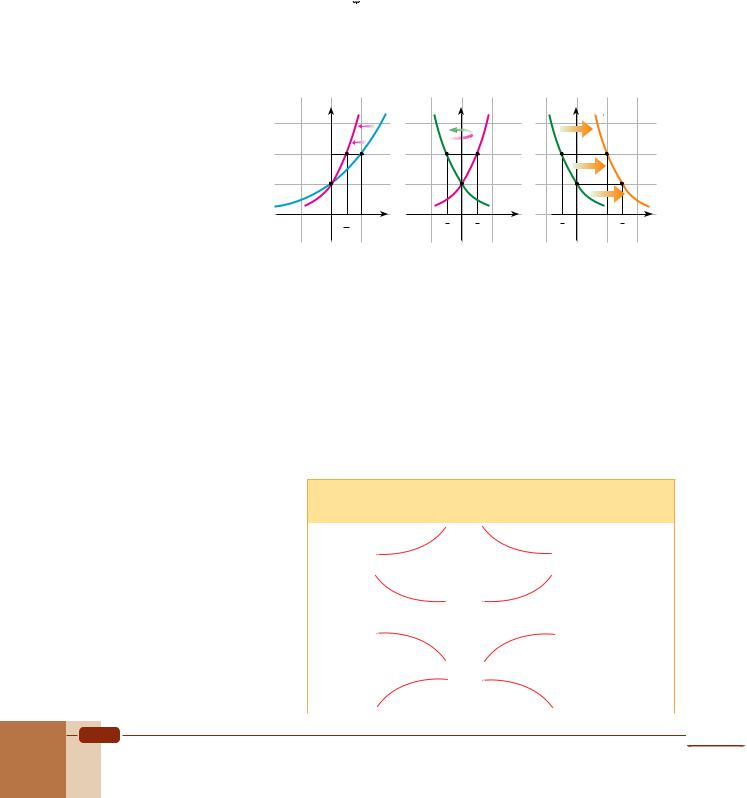
EXAMPLE 19 Sketch the graph of each function and determine its domain, range and asymptote.
a. f(x) = 3 – (21)– x |
b. f(x) = 22 – x |
|
|
|
Solution a. Step 1: Sketch the graph of |
f (x)=( 1)x. |
|
|
|
|
2 |
|
|
|
Step 2: Reflect the graph in the y-axis to obtain the graph of |
g(x)=( |
1)– x = f(–x). |
||
|
|
|
2 |
|
Step 3: Reflect this new graph in the x-axis to obtain the graph of h(x)= –( |
1)– x = – g(x). |
|||
|
|
|
|
2 |
Step 4: Shift this graph three units upward, because
result is the graph of |
f (x)= 3 – ( |
1)x. |
|
|
|
|
|
|||||||
|
|
|
|
|
|
|
|
2 |
|
|
|
|
|
|
|
|
|
|
y |
|
|
|
|
|
|
|
|
y |
|
f(x)=( |
1 |
) |
x 3 |
g(x)=( |
1 )-x |
|
|
|
|
3 |
g(x)=(1 )-x |
|||
2 |
|
|
|
2 |
|
|
|
|
|
|
|
2 |
||
|
|
|
|
|
|
|
|
|
|
|
|
|
|
|
|
|
|
2 |
|
|
|
|
|
|
|
|
2 |
|
|
|
|
|
1 |
|
|
|
|
|
|
|
|
1 |
|
|
|
|
|
|
0.5 |
1 |
|
|
|
|
-1 |
|
0.5 |
1 |
|
|
|
|
|
|
|
|
|
|
|
|||||
|
|
|
|
|
|
|
|
|
|
|
||||
|
|
|
0 |
|
|
x |
|
|
|
|
|
0 |
-0.5 |
x |
|
|
|
|
|
|
|
|
|
|
|
|
|
|
|
|
|
|
-1 |
|
|
|
h(x)=–( |
1 |
) |
-x |
-1 |
|
|
|
|
|
|
|
|
|
2 |
|
|
|
|||||
|
|
|
|
|
|
|
|
|
|
|
|
|
|
|
|
|
|
-2 |
|
|
|
|
|
|
|
|
-2 |
|
|
Steps 1 and 2 |
Step 3 |
y = –( 21)– x +3 = h(x)+3. The
|
|
|
|
3 |
y |
y=3 |
|
|
|
|
|
|
|
|
|||
|
|
|
|
|
|
|
|
|
|
|
|
|
|
2.5 |
|
1 |
-x |
|
|
|
|
|
y=3–( |
|||
|
|
|
|
2 |
2 ) |
|
||
|
|
|
|
1 |
|
|
|
|
|
|
-1 |
|
|
1 |
|
|
|
|
|
|
|
0 |
-0.5 |
|
x |
|
|
|
|
|
|
|
|
|
|
h(x)=–( |
1 |
) |
-x |
-1 |
|
|
|
|
2 |
|
|
|
|
|
|||
|
|
|
|
|
|
|
|
|
|
|
|
|
-2 |
|
|
|
|
Step 4
For g(x) = 2–x,
g(x + 2) = 2–(x + 2) 22 – x.
So f(x) = 3 – (21)– x has domain , range (– , 3) and asymptote y = 3.
 b. We first sketch the graph of f(x) = 2x and reflect it in the y-axis to obtain g(x) = 2–x = f(–x).


 We then need to determine which value to use in f(x) to obtain 22–x. We can use y = g(x – 2) = 2–(x–2) = 22–x. So we need to apply a horizontal shift with p = 2 to the graph of g(x), i.e. we shift the graph of g(x) two units to the right.
domain |
: |
range |
: (0, ) |
asymptote : y = 0
|
|
y |
|
|
2 |
|
|
g(x)=-2x 1 |
f(x)=2x |
||
-1 |
0 |
1 |
x |
|
y |
|
|
|
|
|
2 |
|
y=22-x |
|
|
|
|
|
|
|
|
|
1 |
|
|
|
|
|
g(x)=-2x |
|
|
|
|
-1 |
0 |
1 |
2 |
3 |
x |
130 |
Algebra 11 |
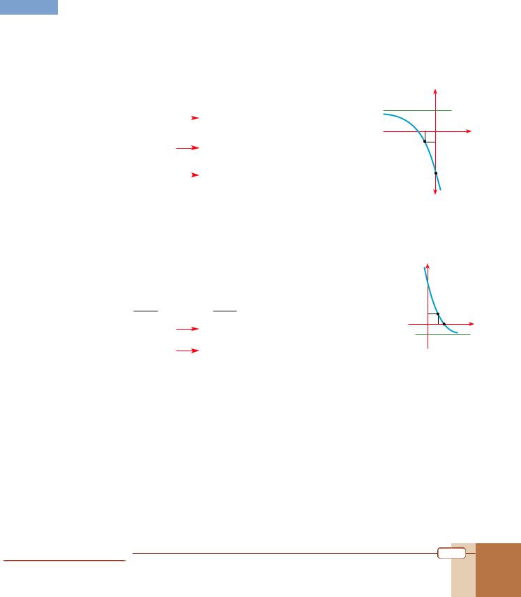
EXAMPLE 20 Sketch the graph of each function and determine its domain, range and asymptote.
|
1 ex |
1 |
a. f(x) = |
b. y = 23 x |
|
|
3 |
|
|
Solution |
a. We first sketch the graph of f(x) = ex, and then shrink it vertically by a factor of |
1 |
, |
||||||||||||||
|
y |
|
|
|
|
|
|
|
|
|
|
|
|
|
|
|
3 |
|
|
|
|
because y = 1 ex = |
1 |
f(x) |
where c= 1. |
Since (0, 1) and (1, e) are two points on y = ex, |
|||||||||||
|
e |
3 |
|
|||||||||||||||
|
|
|
|
3 |
3 |
|
3 |
|
|
|
|
|
|
|
|
|
|
|
|
|
2 |
|
the points |
(0, 1) and |
(1, |
e ) will be on |
y = 1 ex. |
|
|
|
|
|
|
|
|
|
|
f(x)=ex |
|
|
|
|
3 |
|
|
3 |
3 |
|
|
|
|
|
|
|
|
|
|
1 |
|
So the function has domain , range + and asymptote y = 0. |
|
|
|
|
|
|
|
||||||||
|
|
y=1 ex |
|
|
|
|
|
|
|
|
|
|
|
|
|
|
|
|
|
|
3 |
|
|
|
|
|
|
|
|
|
|
|
|
|
|
|
|
|
|
1 |
x |
b. We sketch the graph of f(x) = 2x and |
4 |
y |
(2, 4) |
|
|
(6, 4) |
|
|
||||||
|
|
|
|
apply a horizontal stretch with a |
|
f(x)=2x |
|
|
|
|
|
|
|
|||||
|
|
|
|
|
|
|
|
|
|
|
|
|
||||||
|
|
|
|
factor of 1 |
= 1 = 3 after identifying |
3 |
|
|
|
|
|
1 x |
|
|
|
|||
|
|
|
|
d |
1 |
|
|
|
|
(1, 2) |
|
|
|
y=23 |
|
|
|
|
|
|
|
|
|
3 |
|
|
|
2 |
|
|
(3, 2) |
|
|
|
|
||
|
|
|
|
1 |
|
|
d = 1 . |
|
|
|
|
|
|
|
|
|
|
|
|
|
|
|
y = 23 x = f( 1 x) and |
1 |
|
|
|
|
|
|
|
|
|
||||
|
|
|
|
|
3 |
|
3 |
|
|
|
|
|
|
|
|
x |
|
|
|
|
|
|
In other words, each point (x, y) on |
|
|
|
|
|
|
|
|
|
|||||
|
|
|
|
-1 |
|
1 |
2 |
3 |
4 |
5 |
6 |
|
|
|||||
|
|
|
|
f(x) = 2x will move to (3x, y). |
|
|
|
|||||||||||
|
|
|
|
|
|
|
|
|
|
|
|
|
|
|||||
|
|
|
|
So the function has domain , range + and asymptote y = 0. |
|
|
|
|
|
|
|
|||||||
EXAMPLE 21 Sketch the graph of each function and determine its domain, range and asymptote. a. y = 32x+5 b. y = 23 – 2x
Solution a. We sketch the graph of f(x) = 3x and
write g(x) = 32x = f(2x). We determine
d = 2 and shrink the graph of f(x) by a factor of d1 = 21 . Since
y = 32x+5 = 32 (x+52 ) = g(x+ 52),
|
|
|
y |
|
|
|
3 |
2x |
(1, 3) |
|
g(x)=3 |
|
|
|
|
|
2 |
|
|
f(x)=3 |
x 1 |
|
|
|
|
|
|
||
x |
–1 |
0 |
0.5 |
1 |
|
|
|
|
y |
|
|
(–2, 3) |
|
|
3 |
|
|
|
|
|
|
|
|
y=32x+5 |
|
2 |
|
|
|
|
|
|
|
|
(–2.5, 1) |
|
1 |
g(x)=32x |
||
x |
–2.5 –2 |
–1 |
0 |
0.5 |
1 |
we shift the graph of g(x) 52 units to the left. So the function has domain , range (0, ) and asymptote y = 0.
Exponential and Logarithmic Functions |
131 |
b. Starting with the graph of f(x) = 2x we follow the steps:
Step 1: Shrink |
the |
graph |
horizontally |
by a factor |
of |
1 |
to |
obtain |
the |
graph |
of |
||||
g(x) = 22x = f(2 x). |
|
|
|
|
2 |
|
|
|
|
|
|
||||
|
|
|
|
|
|
|
|
|
|
|
|||||
|
|
d |
|
|
|
|
|
|
|
|
|
|
|
|
|
Step 2: Reflect this graph in the y-axis to obtain the graph of h(x) = 2–2x = g(–x). |
|
||||||||||||||
|
|
|
3 |
|
|
|
|
|
|
2–2( x– |
3 |
|
|
|
|
Step 3: Shift this graph |
units to the right since y =3–2x |
= |
2 ) = h(x – 3). |
|
|||||||||||
|
|
|
2 |
|
|
|
|
|
|
|
|
|
2 |
|
|
|
y |
g(x)=22x |
|
y |
g(x)=22x |
|
y |
y=23 – 2x |
|
|
|
|
|||
|
|
|
|
|
|
|
|
|
|
|
|
|
|||
|
2 |
|
|
|
|
2 |
|
|
2 |
|
|
|
|
|
|
f(x)=2x |
1 |
|
|
|
|
1 |
h(x)=2–2x |
|
1 |
|
|
|
|
|
|
|
|
|
|
|
|
|
|
h(x)=2–2x |
|
|
|
|
|
||
-1 |
|
1 |
1 x |
1 |
|
1 |
|
1 |
1 |
3 |
x |
|
|
|
|
|
-1 - 2 |
|
2 1 x |
- |
2 |
2 |
|
|
|
||||||
|
|
2 |
|
|
|
|
|
|
|
|
|
|
|
|
|
As we can see, applying step-by-step transformations to the basic exponential function f(x) = ax to graph a function y = c ad(x + p) + k is straightforward but it can take a long time. As an alternative approach, we can use a more basic procedure, as follows:
The two points (0, 1) and (1, a) on the graph of f(x) = ax will shift to (–p, c + k) and ( d1 – p, c a+ k) respectively for y = c ad(x + p) + k. By plotting these two points and drawing the horizontal asymptote at y = k, we can obtain a rough graph of y = c ad(x + p) + k. We can
also use the following table:
Graphs of functions of the form y = c ad(x + p) + k
c |
d |
|
a > 1 |
|
0 < a < 1 |
Domain |
Range |
|||
|
|
|
|
|
|
|
|
|
|
|
+ |
+ |
|
|
y = k |
|
|
|
y = k |
|
(k, ) |
|
|
|
|
|
|
|
|
|||
|
|
|
|
|
|
|
||||
|
|
|
|
|
|
|
|
|
|
|
+ |
– |
|
|
y = k |
|
|
|
y = k |
|
(k, ) |
|
|
|
|
|
|
|
|
|
||
|
|
|
|
|
|
|
||||
|
|
|
|
|
|
|
|
|
|
|
– |
+ |
|
|
y = k |
|
|
|
y = k |
|
(– k) |
|
|
|
|
|||||||
|
|
|
|
|
|
|
||||
|
|
|
|
|
|
|
|
|
|
|
– |
– |
|
|
y = k |
|
|
|
y = k |
|
(– k) |
|
|
|
|
|||||||
|
|
|
|
|
|
|
||||
|
|
|
|
|
|
|
|
|
|
|
132 |
Algebra 11 |
EXAMPLE 22 Sketch each graph. |
|
a. y = –3 2x + 1 + 2 |
b. y = 23 – 2x – 1 |
Solution a. By comparing the equation with the general form y = c ad(x + p) + k, we identify c = –3, d = 1, p = 1 and k = 2. So the three points (x, y), (0, 1) and (1, 2) on the graph of f(x) = 2x will move as follows:
f(x) = 2x |
|
|
y = –3 2x + 1 + 2 |
|
|
(x, y) |
|
|
( x |
– p, c y+ k) |
|
|
|
||||
|
|
|
d |
|
|
(0, 1) |
(0 |
– 1, – 3 1+2)=(–1, –1) |
|||
|
1 |
|
|
||
(1, 2) |
|
(1 |
– 1, –3 2+2)=(0, –4). |
||
|
|||||
|
1 |
|
|
||
|
y |
|
|
2 |
y = 2 |
|
1 |
|
-1 |
|
|
|
|
|
|
-1 |
x |
|
|
|
|
-4 |
|
We plot the points (–1, –1) and (0, –4), draw the horizontal asymptote y = k = 2 and then sketch the graph.
b. By rewriting the given equation as y = 23 – 2x – 1 = 2–2( x– 23) – 1, we identify c = 1, d = –2,
p = – |
3 , and k = –1. So the points (0, 1) and (1, 2) on f(x) = 2x will |
|
y |
|
|
|
|
2 |
|
|
|
|
|
move as follows: |
|
|
|
|
|
|
|
f(x) |
y |
|
|
3 |
|
|
|
|
|
1 |
|
|
|
|
( 3 , 0) |
|
2 |
|
|
|
(0, 1) |
|
|
|
||
|
y = -1 |
1 |
2 |
x |
||
|
|
2 |
-1 |
|
|
|
|
|
|
|
|
|
|
|
(1, 2) |
(1, 1). |
|
|
|
|
Using y = –1 as the horizontal asymptote, we plot the points and sketch the graph.
D. APPLICATIONS OF EXPONENTIAL FUNCTIONS
Exponential functions have many applications in the real world. Many of these applications are in physics, biology, electronic engineering, computer technology and economics. Exponential functions are also sometimes used in the social sciences: for example, the popularity of advertisements or fashions often decreases exponentially.
Exponential and Logarithmic Functions |
133 |

Any situation in which the rate of change of a quantity is proportional to the amount present can be modeled by an exponential function. Earlier in this book, we considered the example of a virus spreading through the population of your city. The rate at which the virus spreads is proportional to the number of people infected at a particular time. We can therefore model the spread of the virus with an exponential equation.
We have also seen that exponential functions are either increasing or decreasing. Real-life situations which can be modeled by increasing exponential functions are examples of exponential growth, while situations which can be modeled by decreasing exponential functions are examples of exponential decay.
Both exponential growth and decay can be modeled by an exponential function of the form
P = P0 at.
The value P0 represents the initial quantity that is growing or decaying. This could be an initial number of bacteria, the population of a city at a given time, or the original value of an investment.
a is the constant number and the base. It represents the rate of change. When a 1 there is exponential growth, and when 0 a 1 there is exponential decay. In situations where the growth or decay rate is given as a percentage, we can calculate a as follows:
1. for exponential growth, add the per cent increase to 100% and change the resulting percentage into a decimal.
2.for exponential decay, subtract the per cent decrease from 100% and change the resulting percentage into a decimal.
t is the time interval over which the growth or decay happens, in a given unit (days, years, decades, etc.).
1. Exponential Growth
Exponential growth occurs when a quantity grows by a constant percentage in each fixed period of time. This means that the larger the quantity gets, the faster it grows. Population growth, the spread of a virus and the growth in the number of cells in a bacterial colony are all examples of exponential growth.
Here is a famous story which is based on exponential growth and which shows how its surprising characteristics have fascinated people through the ages.
134 |
Algebra 11 |

The Legend of the Grain of Rice
There was once a clever courtier who presented a beautiful chess set to his king. In return, he asked only that the king place a grain of rice on the first square of the chessboard, and then double the number of grains he placed on each subsequent square. In other words, the king had to place one grain of rice on the first square, two grains on the second square, four grains on the third square and so on.
Since a chessboard has only 64 squares, this seemed to the king to be a modest request, so he called for his servants to bring the rice.
When the king’s men started filling the squares with rice grains, the fun started. Though the eighth square needed only 128 grains, the 22nd square needed roughly 2 million rice grains. The 23rd square needed four million rice grains; the 24th 8 million. And there were still forty squares to go, with the last square needing 9,223,372,036,854,775,808 (roughly 9 million trillion) rice grains! In total, the king should have placed 18,446,744,073,709,551,615 grains on the board (adding up all the squares), which would be 549,755,830,887 tons of rice.
Obviously, the king could not keep his promise. Long before he reached the 64th square, every grain of rice in the kingdom had been used. Even today, the total world rice production would not be enough to meet the amount needed for the final square of the chessboard: the required amount would cover the entire surface of the Earth with rice fields two times over, oceans included. If one grain were counted out every second, it would take 584 billion years (i.e. nearly 130 times the age of the Earth) to count them all.
Square number (n) |
1 |
2 |
3 |
4 |
5 |
... |
n |
... |
64 |
Number of grains |
1 |
2 |
4 |
8 |
16 |
... |
|
... |
|
Formula |
20 |
21 |
22 |
23 |
24 |
... |
2n – 1 |
... |
263 |
|
|
|
|
|
|
|
|
|
|
Obviously the king in the story had not studied mathematics, as he did not understand exponential growth. The secret to understanding the arithmetic is that the rate of growth (doubling for each square) applies to an ever-increasing amount of rice, so the number of grains added at each step goes up, even though the rate of growth is constant.
Exponential and Logarithmic Functions |
135 |
EXAMPLE 23 If the world population was 6.5 billion people in 2005 and if the population continues to grow by 1.5% annually, what will the approximate population be in 2010?
Solution We begin by identifying the values of P0, a and t in the problem.
P0 is the initial quantity. It corresponds to the population of the world in the year 2005: 6.5 billion.
Since the world population grows by a constant percentage (1.5%), we add 1.5% to 100% to obtain 101.5% and then convert 101.5% into decimal number. As a result, a is 1.015.
Since 2010 is five years after 2005, t is 5. Substituting the values into the formula, we obtain
P = P0 at = 6.5 (1.015)5 P = 6.5 1.077 P 7.005. So the world population in 2010 will be approximately 7 billion.
EXAMPLE 24 A colony of bacteria consists of 1000 bacteria. If the bacteria population triples every 30 minutes, what will the population be after 2 hours?
Solution Again we use P = P0 at.
P0 is the initial number of bacteria in the colony (1000).
Since the population triples for each period, we take the rate of growth, a, as 3.
To find t, we first convert two hours into minutes: 2 60 = 120 minutes
and divide this by 30 to identify the number of periods:
t = 12030 = 4.
Now we substitute the values into the formula: P = 1000 34 = 81000.
So after two hours there will be 81000 bacteria in the colony.
136 |
Algebra 11 |

2. Exponential Decay
Exponential decay occurs when a quantity decreases by a constant percentage in each fixed period of time. The decay of radioactive substances is an example of exponential decay.
All radioactive substances have a specific half-life, which is the time required for half of the particular substance to decay. For example, if we have 1000 grams of a substance with a half-life of 10 years, we can express the amount of the substance remaining after a given number of years as follows:
Archaeologists use a method called radiocarbon dating (also called carbon-14 dating) to find out how old archaeological discoveries are. Radiocarbon dating relies on the exponential decay of radioactive carbon-14 atoms in non-living things.
The carbon dioxide in the Earth's atmosphere always contains a fixed percentage of carbon-14 atoms. Plants absorb this carbon-14 with the carbon dioxide, and pass it on to other living creatures through the food chain. As a result, the ratio of normal carbon (carbon-12) to radiocarbon (carbon-14) in the atmosphere and in all living organisms is the same.
When an organism dies, the amount of carbon-12 it contains remains the same, but the carbon-14 decays exponentially with a half-life of about 5730 years. Scientists can therefore use the ratio of carbon-12 to carbon-14 in a non-living organism to find out how long ago it died.
Number of years |
Amount of substance remaining |
||||||||||||||
10 |
1000 |
|
1 |
|
|
|
|
|
|
|
|
|
|
|
|
|
|
|
2 |
|
|
|
|
|
|
|
|
|
|
|
|
20 |
1000 |
|
1 |
1 |
=1000 ( 1)2 |
|
|||||||||
|
|
|
2 |
|
2 |
|
2 |
|
|
|
|
|
|||
|
|
|
|
1 |
|
2 |
|
1 |
|
|
|
1 |
3 |
||
30 |
1000 |
|
( |
2) |
|
|
2 =1000 ( |
2) |
|
||||||
|
|
( |
1) |
t |
|
=1000 2 – |
|
t |
|
||||||
t |
1000 |
10 |
|
10 |
|
|
|||||||||
|
|
|
|
2 |
|
|
|
|
|
|
|
|
|
|
|
|
|
|
|
|
|
|
|
|
|
|
|
|
|
|
|
|
|
|
|
|
N(t)= N 2– |
t |
|
|
|
|
|||||
More generally, we can say that the function |
|
h |
|
|
expresses |
||||||||||
|
|
|
|
|
|
|
|
|
0 |
|
|
|
|
|
|
the amount of a radioactive substance which remains after t years where h is the half-life (measured in the same unit as t) and N0 is the original amount of the substance.
|
25 |
|
|
|
|
|
|
|
|||
EXAMPLE |
An isotope of the synthetic element Californium has a half-life of approximately 45 minutes. |
||||||||||
|
How long would it take for a sample of Californium to decay to 25% of its original mass? |
||||||||||
|
|
||||||||||
Solution |
Let N0 be the original mass of the sample and let t be the desired time (in minutes). |
||||||||||
|
|
25% of N0 means 0.25 N0. Using this value in the formula above gives us |
|||||||||
|
|
|
|
t |
|
t |
|
t |
|||
|
|
0.25 N |
= N 2– |
|
1 = 2– |
|
2–2 = 2– |
|
–2 = – |
t |
t= 90. |
|
|
45 |
45 |
45 |
|||||||
|
|
|
|||||||||
|
|
0 |
0 |
|
4 |
|
45 |
|
|||
|
|
|
|
|
|
|
|||||
So it would take approximately 90 minutes for the sample to decay.
Exponential and Logarithmic Functions |
137 |

If interest is compounded, its amount is based on an initial investment plus any previous interest.
If interest is compoundedannually then n = 1,quarterly then n = 4,monthly then n = 12 in the compound interest
formula.
3. Compound Interest
Compound interest is important to anyone with money in a bank account which earns interest. It is also important in many financial calculations.
If an amount of money P, called the principal, is invested at an annual interest rate r (expressed as a decimal) compounded n times a year, then the amount A in the account at the end of t years is given by
A = P ( + nr )nt .
This formula is often referred to as the compound interest formula.
EXAMPLE 26 You deposit $200 in a bank that pays 7% interest compounded quarterly. Find the amount in the account after 3 years, rounded to the nearest dollar.
Solution After identifying P = 200, r = 7% = 1007 , n = 4 and t = 3, we apply the compound interest formula as follows:
A = P(1+ nr )nt = 200(1+ 0.407)4.3 = 200(1+0.0175)12
= 200(1.0175)12 200 1.23144 = 246.288.
Thus, after 3 years there will be approximately $246 in the account.
|
27 |
|
|||||
EXAMPLE |
$1000 is invested in an account with an interest rate of 9% compounded monthly. Find the |
||||||
|
new principal after 5 years. |
|
|
||||
|
|
|
|
||||
Solution |
Applying the compound interest |
formula with |
|||||
|
|
r = 9% =0.09, n = 12, t = 5 and P = $1000, we find |
|||||
|
|
that the amount after five years is |
|
|
|||
|
|
|
0.09 |
12 5 |
|
60 |
$1565.68. |
|
|
A =1000(1+ |
|
) |
=1000(1.0075) |
|
|
|
|
12 |
|
||||
|
|
|
|
|
|
|
|
138 |
Algebra 11 |