

Interactive Plot Editing
If you enable plot editing mode in the SCILAB figure window, you can perform point-and-click editing of the objects in your graph. In this mode, you select the object or objects you want to edit by double-clicking it. This starts the Property Editor, which provides access to properties of the object that control its appearance and behavior.
Plot editing mode provides an alternative way to access the properties of SCILAB graphic objects. However, you can only access a subset of object properties through this mechanism. You may need to use a combination of interactive editing and command line editing to achieve the effect you desire.
Printing Graphics
You can print a SCILAB figure directly on a printer connected to your computer or you can export the figure to one of the standard graphic file formats supported by SCILAB. There are two ways to print and export figures:
using the Print option under the File menu
using the print command
Printing from the Menu
There are four menu options under the File menu that pertain to printing:
the Page Setup option displays a dialog box that enables you to adjust characteristics of the figure on the printed page.
the Print Setup option displays a dialog box that sets printing defaults, but does not actually print the figure.
the Print Preview option enables you to view the figure the way it will look on the printed page.
the Print option displays a dialog box that lets you select standard printing options and print the figure.
Generally, use Print Preview to determine whether the printed output is what you want. If not, use the Page Setup dialog box to change the output settings. Select the Page Setup dialog box Help button to display information on how to set up the page.
Exporting Figure to Graphics Files
The Export option under the File menu enables you to export the figure to a variety of standard graphics file formats.
5.3.4 3D Plotting
Scilab provides many powerful instructions for the visualization of 3D data. The instructions provided include tools to plot wire-frame objects, 3D plots, curves, surfaces, and can automatically generate contours, display volumetric data, interpolate shading colors. Here are some commonly used functions (there are many more):
plot3, stem3, pie3, comet3, contour3, mesh, meshc,
surf, surfc, sphere, ellipsoid, cylinder.
Among these instructions, plot3 and comet3 are the 3D matches of plot and comet commands mentioned in the 2D plot section.
The 3D plot functions intended for plotting meshes and surfaces 'mesh' and 'surf', and their several variants 'meshc', 'meshz', 'surfc', and 'surfl', take multiple optional input arguments, the most simple form being 'mesh(z)' or 'surf(z)', where z represents a matrix.
Usually, tridimensional curves are represented by the values of z-coordinates samples on a grid of (x,y) values.
Thus, to create a surface or 3D plot we first need to generate a grid of (x,y) coordinates and find the height (z-coordinate) of the surface at each of the grid points. Scilab provides the function 'meshgrid' to create a grid of points over a specified range.
Meshgrid
Suppose that you want to plot the function z = x2 – 10y + 2 over the domain 0 ≤ x ≤ 4 and 0 ≤ y ≤ 4. To do so, we first take several points in the domain, say 25 points, as shown in fig.5.6:
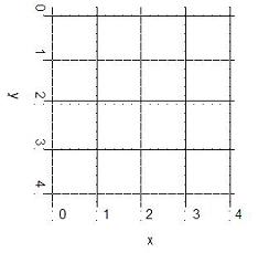
Figure 5.6 - Grid to calculate the function
We can create two matrices x and y, each of size 5 x 5, and write the xy-coordinates of each point in these matrices. We can then evaluate z with the command z = x.^2 – 10*y + 2.
However, creating the two matrices x and y is much easier with the meshgrid command.
>>vx = 0 : 4 % creates vectors x and y, from 0 to 4
vx = 0 1 2 3 4
>>vy = vx
vy = 0 1 2 3 4
>>[x,y] = meshgrid(vx,vy) % creates meshgrid to be used in 3D plot
x = 0 1 2 3 4
0 1 2 3 4
0 1 2 3 4
0 1 2 3 4
0 1 2 3 4
y = 0 0 0 0 0
1 1 1 1 1
2 2 2 2 2
3 3 3 3 3
4 4 4 4 4
The commands shown above generate the 25 points shown in the figure. All we need to do is generate two vectors, vx and vy, to define the region of interest and distribution or density of our grid points. Also, this two vectors do not have to be either the same size or linearly spaced. It is very important to understand the use of meshgrid.
See the columns of x and the rows of y. When a surface is plotted with the 'mesh(z)' command (where z is a matrix), the tickmarks on the x and y axes do not indicate the domain of z but the row and column indices of the z-matrix. Typing 'mesh(x,y,z)' or 'surf(x,y,z)' (where x and y are vectors used by 'meshgrid' to create a grid), result in the surface plot of z, with x and y values shown along the respective axes.
Surf and Surfc
surf(X,Y,Z) creates a shaded surface using Z for the color data as well as surface height. X and Y are vectors or matrices defining the X and Y components of a surface. If X and Y are vectors, length(X) = n and length(Y) = m, where [m,n] = size(Z). In this case, the vertices of the surface faces are (X(j), Y(i), Z(i,j)) triples. To create X and Y matrices for arbitrary domains, use the meshgrid function.
surfc(...) draws a contour plot beneath the surface.
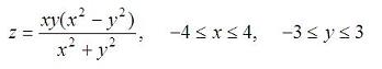
Example 5.1. We'll 3D plot the following surface:
Type following commands:
>> vx = -4 : 0.2: 4;
>> vy = -3 : 0.2: 3;
>> [x,y] = meshgrid(vx, vy); % calculates the necessary grid
>> z = x .* y .* (x.^2 - y.^2) ./ (x.^2 + y.^2 + eps); % calculates z
>> surfc(x,y,z)
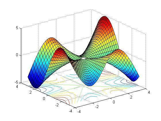
Figure 5.7 – Surface for example 5.1