CHAPTER 7

THE DEVELOPMENT OF GEOMETRY, I

UNFETTERED BY TRADITION, ALGEBRA had made rapid strides during the fifteenth and sixteenth centuries, while geometry, still felt by mathematicians to be in thrall to the towering achievements of the ancient Greeks, had languished. But at the beginning of the seventeenth century geometry was to receive a decisive stimulus through the injection of the methods of algebra. This was occasioned largely through the work of Fermat—in his Ad Locos Planos et Solidos Isagoge, “Introduction to Plane and Solid Loci”, written in 1629 but not published until 1679—and the philosophermathematician Descartes—in his La Géométrie, which appeared as an appendix to his seminal philosophical work Discours de la Méthode of 1637. The major effect of the coordinate—also known as algebraic or analytic—geometry they created was to establish a correspondence between curves or surfaces and algebraic equations, thereby opening up geometric investigation to the powerful quantitative methods of the newly emerged algebra.

COORDINATE /ALGEBRAIC/ANALYTIC GEOMETRY

Algebraic Curves

The fundamental idea of coordinate geometry is to associate with each point P in the Euclidean plane a pair of real numbers (x, y)—the coordinates of P—giving the distances from two intersecting lines—the coordinate, or x- and y-axes—in the plane. The axes are usually taken as being perpendicular—in that case the coordinates are referred to as rectangular—and their point of intersection, that is, the point O with coordinates (0, 0), is called the origin. The first coordinate x of P is called its abscissa (from Latin abscindere, “to cut off”) and the second coordinate y its ordinate (from Latin ordinare, “to put in order”).

x P = (x, y) y

O

111

where none of a, b and p is equal to zero.

Equations 2 and 8 are not satisfied by any real numbers, but only imaginary ones, and accordingly represent imaginary curves. The only real number satisfying equation 3 is the pair (0, 0), and so the corresponding curve is reduced to a single point.

The identification of conic sections with equations of degree two was one of the first significant achievements of coordinate geometry.

Cubic Curves

It was Isaac Newton (1642–1727), later famed for his theory of universal gravitation, who first undertook the systematic investigation of third-degree, or cubic curves. His work on this subject, the Enumeratio Linearii Tertii Ordinii, was actually completed by 1676, but not published until 1704. Newton claimed that all curves represented by the general third-degree equation

ax3 + bx2y + cx 2 + dy3 + ex2 + fxy + gy2 + hx + jy + k = 0

can, by an appropriate choice of coordinate axes, be reduced to one of the following four forms:

I.xy2 + ey = ax3 + bx2 + cx + d

II.xy = ax3 + bx2 + cx + d

III. y2 = ax3 + bx2 + cx + d

IV. y = ax3 + bx2 + cx + d.

James Stirling (1692–1770) published a proof of Newton’s claim in 1717.

Newton also advanced the remarkable claim that all cubic curves could be obtained from those of type III by projecting between planes. This assertion was not formally

established until 1731, when Claude-Alexis Clairaut (1713–1765) and François Nicole

independently published proofs. Clairaut approached the problem by introducing a surface in three-dimensional space (see section on higher-dimensional spaces below) defined by the equation

This surface is a cubic cone made up of the lines joining the origin to the cubic curve of type III in the plane z = 1. Clairaut then established Newton’s assertion by showing that every cubic is the intersection of a plane and a cubic cone of the form (1).

By considering the roots of the right-hand sides of equations I – IV, Newton divided cubics into no less than 72 species. Stirling identified 4 more, and in 1740 another 2 were discovered, giving a total of 78 types, a huge increase over the 9 sorts of conics. Cubics thus form a veritable mathematical zoo.

Returning to the main classification of cubics, I – IV, the most famous curve of type I is the curiously named Witch of Agnesi2, investigated by the Italian mathematician Maria Gaetana Agnesi (1718–1799). This curve has equation xy2 = a2 (a – x) and looks like:

P = (x, y)

Q

A M B

A typical point P on the curve has the property that MQ : MP = AM : AB, where AQB is a circle of diameter a.

A curve with an equation of type II is called a Newton’s trident on account of its three-pronged form:

2 The origin of the name “witch” is intriguing. The curve was discussed by Fermat and, in 1718, the Italian mathematician Luigi Guido Grandi (1671–1742) gave it the Latin name versoria, with the meaning “rope turning a sail,” in accordance with its shape. Grandi also supplied the Italian versiera for the Latin versoria. In her book Instituzioni Analitiche of 1748—the first textbook on the calculus to be written by a woman, and a popular book of its day—Agnesi states that the curve is called la versiera. In his English translation of Agnesi’s book, published in 1801, the British mathematician John Colson (1680–1760) apparently mistook “la versiera” for “l’aversiera”, meaning “the witch,” or “the she-devil.” It is with this name that the curve came to be known in the English-speaking world.

Curves with equations of type III were called by Newton diverging parabolas. He discussed the five forms of the curve which arise from the relations among the roots of the cubic equation in x on the right-hand side of III:

$

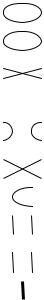
When all the roots of this equation are real and unequal the curve consists of a closed oval and a parabolic branch, as in the first of the figures immediately above. As the two smaller roots approach each other the oval shrinks to a point and the parabolic branch assumes a more bell-like shape, as in the second figure. If the two greater roots are equal, then the curve assumes the shape shown in the third figure, and is then known as a nodated parabola. If all the roots are equal, the curve appears as in the fourth figure, and is then called a cuspidal or semicubical parabola. Finally, if two roots are imaginary, then the curve has only one bell-like branch, as in the fifth figure.

The most familiar cubic curves—the cubic parabolas—are of type IV and look like this:

A higher-degree curve such as a cubic can display certain oddities not found in firstor second-degree curves. In particular it may possess singular points, that is, points at which the tangent to the curve behaves in an anomalous way. The simplest sort of singular point is an ordinary double point or node, where two separate branches

of the curve cross without touching. Here there is not one, but two tangents, each associated with a branch:

Another type of double point is a cusp, at which the two tangents to the separate branches of the curve coincide:

A curve lacking singular points in the sense just described is called nonsingular. Nonsingular cubics of type III with rational coefficients—the so-called elliptic curves— have come to play an important role in number theory, and were, in particular, instrumental in the resolution of Fermat’s Last Theorem (see Chapter 3). Here is the reason in a nutshell. If Fermat’s Last Theorem were false, then there would exist nonzero integers a, b, c and a prime p such that

ap + bp = cp .

It was observed by the German mathematician Gerhard Frey in 1985 that in that event

the associated elliptic curve

y5 = x(x + ap)(x – bp)

would have some rather unlikely properties. Andrew Wiles showed, in a tour de force, that no elliptic curve of this sort could have these properties, and so finally proved Fermat’s Last Theorem.

Another further feature that a curve may possess (although not classified as a singular point) is a point of inflection. At such a point P, the tangent to the curve,

P

imagined as moving along the curve, comes to rest and reverses its direction of motion. Another way of characterizing a point of inflection is the following. A tangent to a curve at a point may be thought of as a line intersecting the curve in no less than two coincident points; the point is a point of inflection if the tangent there intersects the curve in no less than three coincident points. Clairault asserted in 1731 that an irreducible cubic has one, two, or three points of inflection, and Jean-Paul de Gua de Malves (1712–1785) proved in 1740 that in the latter case the inflection points must be collinear. Like the vertices of a polygon, singular points and points of inflection differ from “typical” points on a curve in possessing exceptional features which assist in characterizing the curve.

In the nineteenth century mathematicians came to realize that the properties of algebraic curves could be considerably simplified if these were to be conceived as possessing “points at infinity”, that is, if they were to be regarded as lying in the projective plane (see the discussion of projective geometry later in this chapter). The definition of a singular point on a curve in the projective plane is the same as that for a curve in the Euclidean plane. In the projective plane, a point of inflection is called a flex, and is defined to be a point on a curve at which the tangent intersects the curve in at least three coincident points. It can be shown that every irreducible cubic in the projective plane possesses either a flex or a singular point.

As an example of an assertion about cubic curves which is true in the projective plane, but not in the Euclidean plane, we may consider the following:

The y-axis is tangent to the curve at the origin and so intersects the curve in two coincident points. But it clearly fails to intersect the curve anywhere else in the Euclidean plane. In the projective plane, on the other hand, the “point at infinity” (0, 1, 0) lies both on the curve and on the y-axis.

The fact that (*) holds in the projective plane enables one to derive the single most striking property of an irreducible cubic curve conceived as lying in that plane, namely, that it has the natural structure of an Abelian group. For if P, Q are distinct nonsingular points on an irreducible cubic K, and the line l joining them is not tangent to K at that point, then there is a naturally associated third point PÌQ on K, namely, the

third point at which l meets K. This definition can be extended to any two distinct nonsingular points of K by agreeing that PÌQ = P when l is tangent to K at P, and PÌQ = Q when l is tangent to K at Q. When P and Q coincide, and P is not a flex, then

l

PÌQ

Q

P

l is tangent to K at P and we agree to define PÌQ to be the point where l meets K again. Finally, if P is a flex, we define PÌQ = P. In this way we define a binary operation Ì on the set K* of all nonsingular points of K.

Now fix a point O in K*: O will be called the base point. Define a new binary operation + on K* by

P + Q = (PÌQ)ÌO.

It can be shown that, remarkably, K* is an Abelian group under the operation +, with identity element O, and in which the inverse –P of an element P is given by

–P = PÌ(OÌO). Moreover, the structure of this group depends only on K, and not on the choice of base point O, for it can, again, be shown that the groups arising from different choices of base point are isomorphic.

When K is irreducible, it must possess a flex, and it is advantageous to choose one as base point, because then some basic geometric properties of the curve K have

elegant interpretations in terms of the group structure. For instance, if for n ≥ 1 we write nP for P + P + … + P (n times), then

(a)P + Q + R = O if and only if P, Q and R are collinear;

(b)2P = O if and only if the tangent at P passes through O;

(c)3P = O if and only if P is a flex.

A simple consequence of these facts is that, if P and Q are distinct flexes on an irreducible cubic K, then on the line l joining P and Q there is a third flex of K, which in turn immediately yields de Gua’s theorem that, if a cubic curve has exactly three inflection points, they must be collinear. For choose as base point for K some flex O (which may coincide with P or Q). Then l meets K in a third point R which, by (a) above, satisfies P + Q + R = O, so that R = –P – Q. Now P and Q are both flexes, so by (c) 3P = O = 3Q. It follows that –P = 2P and –Q = 2Q, whence R = 2P + 2Q and 3R = 6P + 6Q = O + O = O. So by (c) R is a flex.

Geometric Construction Problems

Descartes’ ostensible purpose in introducing algebraic methods into geometry was to provide a general method for solving geometric construction problems. The algebraic method transforms a problem of this type into that of solving a system of equations. A construction then turns out to be performable with Euclidean tools only when the corresponding equations can be solved by applying the usual arithmetic operations +, –, × and ÷ together with the extraction of square roots. The equations associated thereby with the ancient problems of doubling the cube and trisecting the angle were shown in the nineteenth century to be insoluble without introducing operations of order higher than square roots (actually, cube roots suffice), so that these problems cannot be solved using Euclidean tools alone. (See Appendix 1 for details.)

A further traditional geometric construction problem which, in the formulation made possible by coordinate geometry, exerted a considerable influence on the development of algebra, was that of constructing a regular polygon of a given number of sides. The ancient Greeks were able, using Euclidean tools, to construct regular polygons of 3, 4, 5, 6, 8 sides, but failed in their attempts to construct one of 7 sides. As we have seen in Chapter 3, the vertices of a regular n-sided polygon are given, in the complex plane, by the solutions to the cyclotomic equation zn = 1. The solutions to this equation are

where ϕ = m.360°/n for m = 1, 2, …, n. Accordingly the regular n-sided polygon is constructible using Euclidean tools exactly when all the solutions z to (1) are so constructible, which in turn will be the case when the cosine of the angle 360°/n is a constructible number (for definition, see Appendix 1). It was shown in the nineteenth century, using the methods of Galois theory, that this is the case just when n has the form

n = 2k. p1. p2. p3 . ...

where each p is a so-called Fermat prime, that is, a prime number of the form 22n +1 . Since neither 7, nor 9, is of this form, neither the regular heptagon nor the regular nonagon is constructible using Euclidean tools.(See Appendix 1 for an elementary proof of the first assertion.)

Higher Dimensional Spaces.

While coordinate geometry in the plane dominated most of its early development, the suggestion of a coordinate geometry in space can already be found in the works of Fermat and Descartes. In his Nouveaux Éléments des Sections Coniques of 1679 the French mathematician Philippe de la Hire (1640–1718) actually took the explicit step of representing a point in space by three coordinates and writing down the equation of a

surface. But the full-scale development of three-dimensional coordinate geometry did not take place until the eighteenth century.

In three-dimensional coordinate geometry three mutually perpendicular axes

Z

x P

y

Y z

O

X

OX, OY and OZ are chosen, and each point P in space is assigned the coordinates (x, y, z), where x, y, z are the distances (taken with the corresponding signs) of the point P from the planes OYZ, OXZ and OXY, respectively. The distance from the point P to a point Q with coordinates (u, v, w) is then given by

Just as an equation F(x, y) = 0 in two variables x, y represents a curve in the plane, so an equation

G(x, y, z) = 0

represents a surface in three dimensional space. A linear equation

ax + by + cz + d = 0

represents a plane. In 1731 Clairault gave the equation

x2/a2 + y2/b2 + z2/c2 – 1 = 0

for the surface of an ellipsoid and showed that an equation which is homogeneous in x, y and z—that is, all terms of the same degree—represents a cone with vertex at the origin. Not long afterwards Jacob Hermann (1678–1733) pointed out that the equation

x2 + y2 = f(z)

represents a surface of revolution about the Z-axis.

The intersection of two surfaces with equations G(x, y, z) = 0 and H(x, y, z) = 0 represents a curve in three-dimensional space. Another way of defining such a curve is to represent it as the trace of the continuous motion of a point. In this case we imagine

the coordinates of a point P on the curve as being given by functions x = x(t), y = y(t), z = z(t) of the variable real number t.

The fact that a plane and space can be “coordinatized” by two or three independent coordinates made it inevitable that the question of the geometric interpretation of larger numbers of coordinates would arise. Thus has arisen the conception of “spaces” of any number of dimensions.

In general, for any natural number n ≥ 1, a point in the n–dimensional Euclidean space En is an n–tuple of real numbers

For 1 ≤ m ≤ n, a set of m equations

F1(x1, …, xn) = 0, … , Fm(x1, …, xn) = 0

determines an n – m dimensional surface in En. In particular, m – 1 such equations determine a 1-dimensional surface, that is, a curve. Another, more widely used method of specifying a curve —as in 3-dimensional space—is again to represent it as the trace of a continuously moving point. Thus the coordinates of a point on the curve are specified by functions x1 = x1(t), …, xn = xn(t) of the variable real number t.

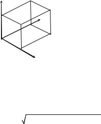
It should be mentioned parenthetically that another, more concrete way of obtaining higher dimensional spaces is to construct them from elements other than points. For example, if we consider our ordinary three-dimensional space to be composed of straight lines rather than points, that is—to employ the striking metaphor of E. T. Bell—as constituting “a cosmic haystack of long thin straws,” as opposed to “an agglomeration of fine birdshot,” then it is four, as opposed to three, dimensional. (This is because a line can be specified by its two points of intersection with two fixed planes, and the specification of each of these points requires two coordinates, making four in all.) This gives rise to the so-called line geometry. Similarly, sphere geometry is obtained by employing spheres as primitive elements: this again yields a fourdimensional space since any sphere may be specified by giving its radius and the three spatial coordinates of its centre.

Higher dimensional spaces have proved of especial importance in physics, where their use often enables a concept to be presented in a suggestive geometric form. A striking instance of this is furnished by the dynamical theory of gases. Suppose that a gas consists of a large number N of molecules. The dynamical state of each of these molecules is then represented by six coordinates, three to specify its spatial position, and an additional three giving its three components of velocity. To describe the state of the gas at any given instant we need to specify all the coordinates of the N molecules in the gas. The resulting 6N coordinates specify the state of the gas, which is thus

can be linked only by an influence travelling faster than light, which, according to the theory of relativity, is impossible. This is reflected in the fact that the interval associated with a spacelike separation would, as the square root of a negative number, be an imaginary quantity.

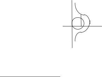
It is illuminating to map out in a “spacetime diagram” the location of events that can be connected by a light ray to a given event e. For simplicity let us suppose that e takes place at the origin (0, 0, 0, 0) of the spacetime diagram. Then if the spatial coordinates of the event f are (x, y, z), its time coordinate t either has the value

or

The graphical presentation of this formula is simplified by confining attention to events f whose z-coordinate is zero. In that case the spacetime diagram may be presented as if it had just two spatial coordinates x and y together with the time coordinate t:

t

x

e

f′

y

g′

Each event in this diagram with lightlike separation from e either lies, like f, on the surface of the future light cone of e (equation 5) or, like f ′, on the surface of the past light cone of e (equation 6). An event such as g contained within the future light cone can be caused by e, and one such as g′ can be the cause of e. On the other hand, an

event such as h which is entirely outside e’s light cone cannot be causally related in any way to e: it is causally independent of e.

In this way coordinate geometry has made possible a remarkable fusion of the concepts of space and time. Through the use of imaginary numbers, Minkowski pushed this fusion to its limit. He introduced a new quantity w to measure time, defined by

w = ict,

or

∆w = ic∆t.

In that case the expression (4) for the squared interval becomes

d(e, e′)2 = (∆x)2 + (∆y)2 +(∆z)2 + (∆w)2,

which is precisely the expression for the squared distance in 4-dimensional Euclidean space. Minkowski was sufficiently impressed by this fact to write the famous words:

Henceforth space by itself, and time by itself, are doomed to fade away into mere shadows, and only a kind of union of the two will have an independent reality.

NONEUCLIDEAN GEOMETRY

Euclid’s postulates were put forward as a body of assertions about lines and points conceived as lying in physical space whose correctness would be immediately obvious to everyone. There is one postulate, however, whose correctness is by no means obvious. This is the fifth—or parallel—postulate which, in Playfair's (John Playfair, 1748–1819) formulation, states that through any point not on a given line one and only one line may be drawn parallel to the given line. The striking feature of this postulate is that it makes an assertion about the whole extent of a straight line, imagined as being extended indefinitely in either direction; for two lines are defined to be parallel if they never intersect, however far they are produced. Now of course there are many lines through a point which do not intersect a given line within any prescribed finite distance, however large. Since the maximum possible length of an actual ruler, thread, or even light ray visible through a telescope is certainly finite, and since within any finite circle there are infinitely many straight lines passing through a given point and not intersecting a given straight line, it follows that the postulate can never be verified —or even refuted—by experiment. On the other hand, all the other postulates of Euclidean geometry have a finite character in that they deal with bounded portions of lines and planes. The fact that the parallel postulate is not experimentally verifiable, while the remaining postulates are, suggested the idea of trying to derive it from the latter. For centuries, mathematicians strove without success to find such a derivation.

One of the first attempts in this direction was made by Proclus (4th century B.C.), who tried to dispense with the need for a special parallel postulate by the ingenious expedient of defining the parallel to a given line to be the locus of all points at a fixed distance from the line. Unfortunately, it then became necessary to show that the locus of such points is indeed a straight line! Since this assertion is actually equivalent to the parallel postulate, Proclus made no real advance here.

Not until 1733 was the first truly scientific investigation of the parallel postulate published. In that year there appeared the book Euclides ab onmi naevo vindicatis— “Euclid Freed of Every Flaw”—by the Italian Jesuit Girolamo Saccheri (1667–1733). Without using the parallel postulate, Saccheri easily showed that if, in a quadrilateral ABCD, the angles at A and B are right angles and sides AD and BC are equal, then the

angles at D and C are also equal. There are then three possibilities: the angles at C and

D are equal acute, right, or obtuse angles. Saccheri showed, assuming that straight lines are indefinitely extensible, that the case of obtuse angles is impossible

(using, of course, the remaining postulates of Euclidean geometry). His aim was then to demonstrate that the acute angle hypothesis also leads to a contradiction, thus leaving the right angle case, which is easily shown to be equivalent to the parallel postulate. Saccheri’s method was thus to assume the acute angle hypothesis, together with the postulates of Euclidean geometry apart from the parallel postulate and attempt to derive a contradiction, a successful outcome showing the parallel postulate to be a consequence of the remaining ones. Remarkably, in the course of his investigations, Saccheri derived many of the theorems of what was later to become known as noneuclidean geometry. Unfortunately, however, he completed his discussion by deriving an unconvincing “contradiction” involving a nebulous idea of “infinite element”. Had he not been so eager to exhibit a contradiction here, but had rather admitted his inability to find one, Saccheri would today indisputably be credited with the discovery of noneuclidean geometry. Nevertheless, despite its lack of boldness, Saccheri's work, along with that of Johann Heinrich Lambert (1728–1777) and AdrienMarie Legendre (1752–1833), suggested the possiblity of a new geometry in which the parallel postulate was no longer affirmed.

At that time, any geometric system not absolutely in accordance with Euclid’s would have been regarded as nonsensical. However, their continual failure to find a proof of the parallel postulate finally convinced mathematicians that it must be truly independent of the others, and that therefore a self-consistent noneuclidean geometry is conceivable.

Janos Bolyai (1802–1860) and Nikolai Ivanovich Lobachevsky (1793–1856) were the first to publish, independently, in 1832 and 1829, respectively, detailed accounts of a system of noneuclidean geometry4. This Bolyai-Lobachevsky—also known as hyperbolic— geometry possesses certain curious features that set it apart from Euclidean geometry in a most dramatic way, and which fully justify Bolyai’s description of it as a “strange new universe”. To begin with, there is always more than one straight line parallel to a given one passing through a given point outside it. Let us examine this situation a little more closely. Calling the given line l and the point P, drop perpendicular PQ to l and let m be the perpendicular through P to PQ. Consider one ray PS of m and various rays between PS and PQ. Some of these rays, such as PR, will

4 Both were in fact anticipated by Gauss, who, however, fearing critical reaction—to which he referred as “the cries of the Boeotians”—, never published his discoveries in noneuclidean geometry.

126 CHAPTER 7

intersect l, while others, such as PY, will not. As R recedes indefinitely on l from Q, PR

l

Q

about PQ. The angle QPX = QPX′is called the angle of parallelism at P with respect to l: the size of this angle depends only on the distance d from P to Q, and not on the identity of the particular line l , nor on that of the particular point P. As the distance d varies, the angle of parallelism α takes on all values between 0 and 90 degrees: as P approaches Q, α approaches 90°, and as P recedes to infinity from Q, α approaches 0°.

Triangles also behave oddly in Bolyai-Lobachevsky geometry. All triangles have angle sum less than 180°, so that, if we define the defect of a triangle to be the difference between 180° and the sum of its angles, the defect of any triangle is always positive. As a triangle shrinks, however, its defect becomes arbitrarily small. Another striking fact about triangles in Bolyai-Lobachevsky geometry is that all similar triangles are congruent. This means that a given triangle cannot be enlarged or shrunk without changing its shape. A startling consequence is that a segment can be determined with the aid of an angle: for example, an angle (50°, say) of an equilateral

triangle determines the length of the side uniquely. To put it more dramatically, BolyaiLobachevsky geometry has an absolute measure of length. This contrasts starkly with Euclidean geometry. For while it shares with Bolyai-Lobachevsky geometry the feature of possessing an absolute measure of angle in the form of the right angle, there can be no absolute measure of length in Euclidean geometry since there the geometric properties of figures are invariant under change of scale.

A further curious feature of Bolyai-Lobachevsky geometry is that all convex quadrilaterals have angle sum less than 360°: in particular, there are no quadrilaterals containing four right angles, that is, there are no rectangles or squares. Since the customary system of measuring area is based on square units, this makes the task of defining area a somewhat ticklish affair. In fact the only reasonable way of defining the area of a triangle is to make it proportional to the defect. Since the defect can never exceed 180°, there is an upper bound to the area of a triangle.

Although Lobachevsky actually showed, by formal methods, that his geometry was consistent, this fact seems to have gone unrecognized at the time. The consistency of Bolyai-Lobachevsky geometry was not in fact publicly affirmed until Cayley, Eugenio Beltrami (1835–1900), Felix Klein (1849–1925) and others constructed models for it, that is, interpretations under which all its postulates could be seen to be true. In Klein's model we take a fixed circle C in the Euclidean plane and interpret point as point in C, line as line in C, and, glancing at the figure below, distance between P and Q as

T

Q

P

S

a certain function of P and Q—actually the logarithm of the cross-ratio (QPST)— which becomes arbitrarily large as P approaches S or Q approaches T. This latter fact ensures that the “lines” in the model can be indefinitely “extended”. In this model the parallel postulate obviously fails—there being many “lines” passing through a given point “parallel” to a given “line” in the sense that they fail to intersect within C. On the other hand the distance function can be chosen in such a way as to ensure that the other postulates of Euclidean geometry remain true.

The Klein model shows that the geometry of Bolyai and Lobachevsky is as consistent as that of Euclid. But which of the two is to be preferred as a description of the geometry of the real world? Notice that we can never determine by experiment whether there are one, or many, lines through a given point parallel to a given line. However, in Euclidean geometry the sum of the angles of a triangle is always 180° , while in Bolyai-Lobachevsky geometry it is always less than 180°. In the nineteenth century Gauss actually performed an experiment to determine which of these alternatives held. But although the result was, within the limits of experimental error, 180°, nothing was settled since, for small triangles (i.e. of terrestrial dimensions), the

deviation from 180° might be so small as to be experimentally undetectable. That is, Bolyai-Lobachevsky and Euclidean geometry, although differing in the large, may coincide so closely in the small as to be empirically equivalent. So far as local properties of space are concerned, then, the choice between the two geometries can be made solely on the basis of simplicity and convenience.

The revolutionary importance of the discovery of noneuclidean geometry lay in the fact that it toppled Euclid's system as the immutable mathematical framework into which our knowledge of objective reality must be fitted.

While the mathematician may regard a “geometry” as being defined by any consistent set of postulates about “points”, “lines”, etc., the physicist will only find the result useful when the postulates in question conform with the behaviour of entities in the real world. Consider, for example, the statement light travels in a straight line. If this is regarded as the physical definition of a straight line, then the postulates of geometry must be chosen so as to correspond with the actual behaviour of light rays. The French mathematician Henri Poincaré (1854–1912) imagined a world confined within the interior of a circle C, in which the velocity of light at each point is inversely proportional to the distance of the point from the circumference of C (for example, C could be made of glass of suitably varying refractive index). It can then be shown that light rays will assume the form of circular arcs perpendicular at their extremities to the circumference of C, and thus that Bolyai-Lobachevsky geometry will prevail. Nevertheless, we can also arrange for Euclidean geometry to apply in this world: instead of regarding light rays as “noneuclidean” straight lines, we simply take them to be Euclidean circles normal to C. Thus we see that different geometries can describe the same physical situation, provided that physical entities (in the case just considered, light rays) are correlated with different notions in the geometries concerned.

In both Bolyai-Lobachevsky and Euclidean geometry it is tacitly assumed that lines can be indefinitely extended. But after Bolyai and Lobachevsky had revealed the possibility of constructing new geometries, it became natural to ask whether noneuclidean geometries could be constructed in which “straight lines” are not infinite, but finite and closed. Such geometries were first considered in 1851 by Georg Friedrich Bernhard Riemann (1826–1866). It turns out that geometries with closed finite lines can be constructed in a completely consistent way: we take as our “space” the surface S of a sphere in which we define straight line to mean great circle on S. Since every pair of great circles intersect (in two points), in this model there are no “parallel lines” at all.

Riemann extended the idea of his geometry by considering a “space” consisting of an arbitrary curved surface, and defining a “straight line” between two points on the surface to be the curve of shortest length or geodesic on the surface joining the points. In this case the deviation of the geodesics from Euclidean straightness provides a measure of the curvature of the surface. Riemann also extended this idea to three (and higher) dimensions, considering a geometry of (real) space analogous to the geometry of a surface, in which the curvature may change the character of the geometry from point to point. This is discussed further in the next chapter.