When you study this diagram (Figure 5.5) carefully youʼll see that the spherically expanding radiation pattern crosses the bottom of this particular antenna at the most negative part of the signal. For a sine wave this would be the 225º point. Notice that the radiated signal crosses the top of the antenna at the most positive part of the signal (the 45º point). The antenna is now receiving an equal, but oppositely charged input and the wave peak cancels the wave valley and the net signal to the receiving antenna is zero. This would be a very bad thing to have happen to your antenna since if you physically placed your receiving antenna at the point in the transmission path where the situation just described was happening, then you would not be able to communicate because the out-of-phase signals would cancel each other.

The reason that this is an impossible scenario is based first on the fact that weʼre talking about near field effects and youʼre probably not going to have a receiver within the near field of a transmitter in the 802.11 wireless LAN environment. This is because at 2.4 GHz or 5.8 GHz the near field is very, very small. How do we know that weʼre talking about near field effects? What we just described related to the spherical wave propagation (4πr2) and that means weʼre talking about effects in the near field. Weʼre going to see that the near field is so small that its significance is appreciated mostly by antenna designers and physicists, and not by engineers working with real-world equipment in realworld 802.11 wireless networks. In the far field, as weʼll discuss shortly, the wave propagation is considered to act like a planar surface, and not like a spherical one.

The Boundary Between the Near Field and the Far Field

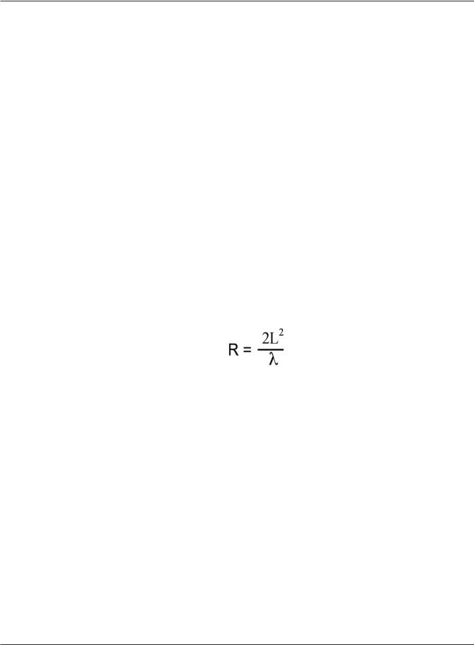
The boundary between the near field and the far field is at a distance R (in meters) from the source that can be approximated with the equation below.

In this equation L is the length of the antenna in meters and, of course, λ is the wavelength of the signal, also in meters. “R” (the boundary distance in meters) is called the Rayleigh distance. The equation is derived by considering a spherical propagation pattern that has expanded to a sphere that is sufficiently large that the wavefront that impinges on the tip of a receiving antenna is 22.5º (π/8 radians) out of phase with the wavefront in the middle of the antenna. This is considered to be a sufficiently “flat” surface of the spherical wavefront so as to consider it as if it were simply a planar surface. To get an idea of why this is true, consider Figure 5.6 below. In this figure youʼll see

the propagating signal considered at three separate angles: 0º, 8º, and 17º. These angles were chosen simply to make comparing and contrasting the wave phases clear. There is no special significance to these angles.

Copyright 2003 - Joseph Bardwell

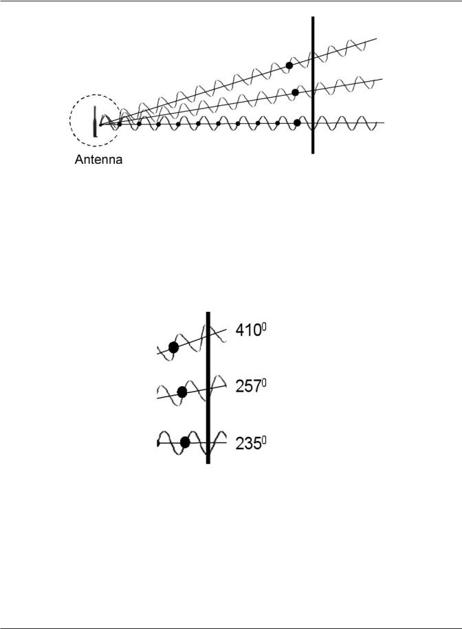
Figure 5.6 Out of Phase Signals Meeting a Vertical Antenna

On the 0º line you see that the start of each frequency cycle has been marked with a dot to serve as a point of reference. The large dot represents the start of the same cycle on all three paths. From this you can see, as we discussed earlier, that the vertical antenna intersects the spherical propagation field at different points for each angle.

One individual frequency cycle is measured in degrees, with a full cycle being equal to 360º. A sine wave peaks at 90º and hits its lowest value at 235º. A close examination of the three waves in Figure 5.6 is shown below in Figure 5.7.

Figure 5.7 A Close View of the Out of Phase Waves

Notice how the 0º (bottom) wave hits the antenna at the lowest point in the cycle, the 235º point. The 8º (middle) wave hits at 257º, and the 17º wave (top) actually hits the antenna in the next cycle. 410º is one full cycle (360º) plus another 50º. You can see that the antenna appears to be hitting the cycle just beyond the initial crest that cycles at 45º, hence it looks like 410º is a good approximation at the point.

An 802.11 access point typically uses a 1-wavelength antenna so L and λ are both equal to 12.5 cm. In this case 2L2/λ = 25 cm (roughly 10 inches). You can see why weʼre interested in the far field for all practical purposes.

Copyright 2003 - Joseph Bardwell