3.3 Ordinary Differential Equations

3.3 Ordinary Differential Equations

Consider the following description of a linear time-invariant dynamical system

where u is the input and y the output. The system is of order n order, where n is the highest derivative of y. The ordinary differential equations is a standard topic in mathematics. In mathematics it is common practice to have bn 1 and b1 b2 . . . bn−1 0 in D3.5E. The form D3.5E adds richness and is much more relevant to control. The equation is sometimes called a controlled differential equation.

The Homogeneous Equation

If the input u to the system D3.5E is zero, we obtain the equation

which is called the homogeneous equation associated with equation D3.5E. The characteristic polynomial of Equations D3.5E and D3.6E is

The roots of the characteristic equation determine the properties of the solution. If ADα E 0, then yDtE Ceα t is a solution to Equation D3.6E.

If the characteristic equation has distinct roots α k the solution is

k 1

where Ck are arbitrary constants. The Equation D3.6E thus has n free parameters.

Roots of the Characteristic Equation give Insight

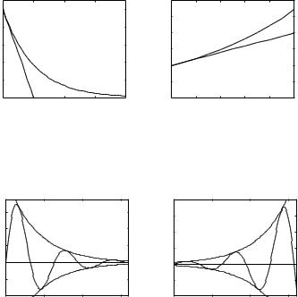
A real root s α correspond to ordinary exponential functions eα t. These are monotone functions that decrease if α is negative and increase if α is positive as is shown in Figure 3.3. Notice that the linear approximations shown in dashed lines change by one unit for one unit of α t. Complex roots s σ iω correspond to the time functions.

which have oscillatory behavior, see Figure 3.4. The distance between zero crossings is π /ω and corresponding amplitude change is eσπ /ω .

77

Figure 3.3 The exponential function yDtE eα t. The linear approximations of of the functions for small α t are shown in dashed lines. The parameter T 1/α is the time constant of the system.

Figure 3.4 The exponential function yDtE eσ t sin ω t. The linear approximations of of the functions for small α t are shown in dashed lines. The dashed line corresponds to a first order system with time constant T 1/σ . The distance between zero crossings is π /ω .

Multiple Roots

When there are multiple roots the solution to Equation D3.6E has the form

k 1

Where CkDtE is a polynomial with degree less than the multiplicity of the root α k. The solution D3.9E thus has n free parameters.

The Inhomogeneous Equation – A Special Case

The equation

78

The solution D3.11E is thus a sum of two terms, the general solution to the homogeneous equation and a particular solution which depends on the input u. The solution has n free parameters which can be determined from initial conditions.

The Inhomogeneous Equation - The General Case

The Equation D3.5E has the solution

The solution is thus the sum of two terms, the general solution to the homogeneous equation and a particular solution. The general solution to the homogeneous equation does not depend on the input and the particular solution depends on the input.

Notice that the impulse response has the form

k 1

It thus has the same form as the general solution to the homogeneous equation D3.9E. The coefficients ck are given by the conditions D3.12E.

The impulse response is also called the weighting function because the second term of D3.13E can be interpreted as a weighted sum of past inputs.

79

Chapter 3. Dynamics

The Step Response

Consider D3.13E and assume that all initial conditions are zero. The output is then given by

The function H is called the unit step response or the step response for short. It follows from the above equation that

The step response can easily be determined experimentally by waiting for the system to come to rest and applying a constant input. In process engineering the experiment is called a bump test. The impulse response can then be determined by differentiating the step response.

Stability

The solution of system is described by the ordinary differential equation D3.5E is given by D3.9E. The solution is stable if all solutions go to zero. A system is thus stable if the real parts of all α i are negative, or equivalently that all the roots of the characteristic polynomial D3.7E have negative real parts.

Stability can be determined simply by finding the roots of the characteristic polynomial of a system. This is easily done in Matlab.

The Routh-Hurwitz Stability Criterion

When control started to be used for steam engines and electric generators computational tools were not available and it was it was a major effort to find roots of an algebraic equation. Much intellectual activity was devoted to the problem of investigating if an algebraic equation have all its roots in the left half plane without solving the equation resulting in the RouthHurwitz criterion. Some simple special cases of this criterion are given below.

∙ The polynomial ADsE s a1 has its zero in the left half plane if a1 0.

∙The polynomial ADsE s2 a1s a2 has all its zeros in the left half plane if all coefficients are positive.

80

3.3 Ordinary Differential Equations

∙The polynomial ADsE s3 a2s2 a3 has all its zeros in the left half plane if all coefficients are positive and if a1a2 a − 3.

Transfer Functions, Poles and Zeros

The model D3.5E is characterized by two polynomials

ADsE sn a1sn−1 a2sn−2 . . . an−1s an

BDsE b1sn−1 b2sn−2 . . . bn−1s bn

The rational function

is called the transfer function of the system.

Consider a system described by D3.5E assume that the input and the output have constant values u0 and y0 respectively. It then follows from D3.5E that

an y0 bnu0

which implies that

y0 bn GD0E u0 an

The number GD0E is called the static gain of the system because it tells the ratio of the output and the input under steady state condition. If the input is constant u u0 and the system is stable then the output will reach the steady state value y0 GD0Eu0. The transfer function can thus be viewed as a generalization of the concept of gain.

Notice the symmetry between y and u. The inverse system is obtained

by reversing the roles of input and output. The transfer function of the

BDsE ADsE system is ADsE and the inverse system has the transfer function BDsE.

The roots of ADsE are called poles of the system. The roots of BDsE are called zeros of the system. The poles of the system are the roots of the characteristic equation, they characterize the general solution to to the homogeneous equation and the impulse response. A pole s λ corresponds to the component eλt of the solution, also called a mode. If ADα E 0, then yDtE eα t is a solution to the homogeneous equation D3.6E.

Differentiation gives

dk y α k yDtE dtk