Petri EC signal deconvolution

1. INTRODUCTION

Steam generators have a long history of being a troublesome major component in pressurized water reactor nuclear power plants, and steam generator tube failures remain a costly concern for nuclear utilities.(1,2) The thousands of thin-walled tubes of a steam generator form a containment boundary between the high-pressure primary and low-pressure secondary water systems. Cracking in an aggressive steam generator environment reduces the structural integrity of the tubing and can lead to tube bursting under the differential water pressure. Therefore, plant operators must repair or plug tubes if significant cracking is detected. Tube cracking has led directly to the decommissioning and replacement of many U.S. steam generators.(3)

1 Argonne National Laboratory, Argonne, Illinois 60439.

149

Eddy current (EC) techniques are currently the predominant technology used for the in-service inspection of nuclear power plant steam generator tubing in the U.S. and elsewhere.(4,5) Current EC measurement techniques using differential bobbin-coil probes are extremely sensitive to the presence of axial cracks in the tube wall, but they are equally sensitive to the presence of dents, fretting, support structures, corrosion products, and other artifacts. EC signal interpretation is further complicated by cracking geometries more complex than a single axial crack. Since cracks are difficult to distinguish from artifacts and even more difficult to characterize, operators are often forced to repair or plug a tube upon detection of a defect, regardless of its effect on tube integrity.(6–8)

One would expect the amplitude and phase delay of an eddy current crack signal to be directly related to the severity of cracking and, thus, to the tube integrity, but attempts to predict tubing burst pressure have been frus-

150

trated by the inability to interpret complicated EC signals. In this work, a signal processing technique has been designed to reconstruct from a raw EC measurement the voltage signal due solely to a crack, filtering out signals from other sources. Through this signal deconvolution technique, the amplitude and phase information of the reconstructed crack signal provide an improved artificial neural network correlation of steam generator tubing burst pressure to EC inspection data.

2. BACKGROUND

2.1. Eddy Current Bobbin-Coil Probes

Periodic inspection of nuclear plant steam generators is required to ensure the integrity of the tubing. During plant shutdown periods, the steam generators can be opened and probes can be extended along the inside of the tubes. Because of their high speed and reasonable reliability, eddy current bobbin-coil probes are the primary examination tool for steam generator tubing.(9) Various other probe designs (rotating pancake coils, pancake arrays, cross-wound coils, transmit/receive reflection coils, etc.) can better characterize defects and are used to help resolve questionable bobbin probe readings, but their slow speeds limit their use for routine inspections.

An EC bobbin coil probe consists of two axially wound coils separated by a small distance.(10) These coils induce an eddy current within a tube wall that flows circumferentially. The induced current produces a secondary magnetic field that opposes and weakens the primary field of the probe coils. That weakening can be measured as a change in the impedance of the coils. Axial defects disrupt the eddy current flow, reducing the secondary magnetic field, and, thus, increasing the coil impedance. Eddy current flow is relatively unaffected by circumferential cracks. The coils can be used to take absolute eddy current measurements, or they can be wired differentially. In the differential mode, a signal is generated only when the two coils encounter different material conditions. In this way, the bobbin probe does not react to smooth changes along the length of the tube, such as due to steady thickness changes or magnetic permeability changes, nor is the probe much affected by probe motion or temperature variations. On the other hand, a differential probe is very sensitive to sudden changes in material conditions, such as at the tip of an axial crack. EC measurements are taken at various ac frequencies to obtain crack depth information, since lower frequencies penetrate deeper into the tube wall:

where v denotes the test frequency, mr denotes the relative magnetic permeability of the metal, and s denotes its conductivity.(11)

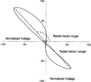
During EC bobbin probe testing, measurements are made of a tube standard with flat-bottom holes of prescribed depths.(12) The amplitude and phase of the EC signal from the steam generator tube inspection are normalized based on the results from the standard tube. The normalized in-phase and quadrature components of the differential signals (i.e., the “horizontal” and “vertical” components) can be combined as a root mean square (RMS) to determine the total voltage at each axial position along the steam generator tube. Plotting the in-phase component versus the quadrature component of the differential signal results in an impedance-plane trajectory, or Lissajous pattern. For a single axial crack in the absence of artifacts, a Lissajous pattern is typically a two-lobed figure eight.(10) Figure 1 shows, for example, the pattern for a steam generator tube with an axial crack. The orientation and shapes of the two Lissajous-pattern lobes are related to the flaw size and type. One characteristic signal feature, for instance, is the radial vector length, which is defined as the distance between the ends of the Lissajous pattern lobes. The angles that the lobes make with respect to the horizontal axis (the radial vector angles) depend on the phase delay of the signal, which, among other things, is related to the depth of the flaw. Complex crack-

Fig. 1. 100 kHz Lissajous pattern for a cracked tube without a tube support plate illustrating the definitions of the radial vector length and radial vector angle.

ing patterns, tube fretting, the presence of tube support structures, and other variables frequently produce complicated Lissajous plots that are not a simple figure eight. In these cases it can be difficult, if not impossible, to identify lobes associated with the dominant crack.

2.2.The Use of Eddy Current Measurements to Assess Tubing Integrity

Current analysis techniques based on EC bobbinprobe measurements have been relatively successful in detecting cracks, but fail almost completely when applied to the characterization of cracks and their effect on tube integrity. For example, EC inspection software is available to linearly mix signals taken at different frequencies.(10) These mixing algorithms can accentuate signals from defects, aiding defect detection, but signal distortions due to mixing make this technique less useful for defect sizing. Since they respond only to an aggregate disruption of electrical current along the circumference of a tube at a given axial position, bobbin coils cannot differentiate multiple defects along the tube circumference. Bobbin probes, therefore, are ineffective for characterizing complex cracking. On the other hand, since bobbin probes respond to the net extent of cracking in a tube, efforts to predict tube burst pressure have been a more promising way to assess tube integrity than through attempts to characterize and size defects. For this reason, the nuclear industry has proposed replacing the crackdepth criterion for removing steam generator tubes from service with one based on EC voltage, arguing that the EC voltage is a better indicator of tube failure.(2,3,8)

Eddy current signals from cracks, wastage, and other physical sources have similar, if not identical, frequency responses. Frequency-based signal processing techniques such as Fourier filtering and wavelet transformations are ineffective at winnowing out artifact signals, since their frequency signatures are indistinguishable from those of crack signals. Nevertheless, Fourier filters, wavelet transforms, and independent component analysis are useful for filtering out electronic noise and noise due to probe wobble.(13–16)

EC based expert rules have been used, with some success, to create algorithms for the identification of defects in steam generator and heat exchanger tubing.(13,17,18) Attempts to use expert systems to estimate the depth of steam generator tubing flaws in tube support plate regions based on EC voltages and phase angles have been less successful.(6) Complex defect morphologies limited the accuracy of those algorithms to only 620% of the tube wall thickness. Even ignoring that large uncertainty, the prediction of crack depth alone may not ade-

quately express the tube’s integrity (i.e., its burst pressure). It is not surprising, then, that current EC-based expert rules have resulted in poor decisions about whether to plug suspect steam generator tubes.(19)

Artificial intelligence methods have the potential for providing improved modeling of tube defects compared to conventional empirical modeling techniques. Beginning in the late 1970s, for example, Doctor, et al.,(20) used pattern-recognition algorithms to determine which EC Lissajous-pattern features best correlated with the defect classification of tubes with electrodischarge-machined (EDM) slots, machined elliptical wastage, and uniform thinning. Their parametric study considered many signal features based on the shape of the Lissajous figures and ones based on the vertical component of the EC voltage readings. Along with classifying the simulated flaws, the researchers attempted to predict the depth of the uniform thinning based on a least-squares regression of EC features. Later attempts to predict the size of the axial slots were largely unsuccessful.(21)

More recently, Jarmulak, et al.,(22) have applied the artificial intelligence technique of case-based reasoning to the classification and characterization of flaws detected through EC inspection and other nondestructive examination methods. Case-based reasoning relies on a comparison of input features (as from an eddy current measurement) to values used previously for training the system. Cases with similar input features would be expected to have similar solutions (e.g., tube burst pressures). Although case-based reasoning has potential advantages over other artificial intelligence techniques, it requires a large data base to cover the range of possible input-feature combinations, especially for problems that depend on several input variables. Case-based reasoning is particularly vulnerable to the effect of data noise. Input data distorted by the presence of artifacts can baffle the analysis system’s attempt to find a matching comparison case in the data base.

2.3.Artificial Neural Network Modeling of Steam Generator Tube Defects

Artificial neural networks (ANNs) have the ability to accurately model complicated, nonlinear relationships even when the underlying analytic functions are unknown.(23,24) Feed-forward multilayer ANNs are organized into multiple layers of nodes that connect input data to corresponding output data.(25) Each node performs a mathematical operation on weighted input it receives from nodes in a previous layer. The output from the node, in turn, becomes input for each node in the subsequent layer. The layers of nodes represent the nonlinear relation-

ships between the input and output data. Training is the process of adapting the connection weights between nodes in response to a set of input signals to optimize the network predictions. That is, the ANN is presented with matched sets of input signals and known output values. Weights are adjusted iteratively until the ANN predictions for all training cases match the known output within a specified convergence criterion. An alternative approach is for the ANN to train for a fixed number of iterations, regardless of how closely the predictions match the known output. Testing consists of comparing predictions of a trained ANN to known output for cases that were not used for training. The ANN may or may not then be reconfigured to optimize the prediction results.

Artificial neural networks are a particularly promising artificial intelligence tool for modeling steam generator tube integrity. ANN techniques have previously been applied to the eddy current identification of flaws in flat plates.(26,27) Similar neural network defect-identification studies using tubes with machined flaws were performed by Udpa and Udpa(28) and by Komatsu, et al.(29) Researchers at Oak Ridge National Laboratory used ANNs to characterize the defect depth and artifact type for tubes with drilled holes and artifacts such as tube supports, copper, and magnetite.(30–32) The Oak Ridge research was later extended to estimate the depth of laboratory-gener- ated outer-diameter stress corrosion cracks in simulated steam generator tubes.(33) Employing the same drilledhole data, researchers at the University of Tennessee applied ANNs to eddy current signal analysis for defect classification and for defect sizing.(34,35) To separate EC crack signals from those due to the artifacts, a reference signal was subtracted from the test signal, where the reference signal was obtained from a tube without holes. In that way, the common features of the two EC measurements were removed, and the hole effects in the test

signal were enhanced. Despite these limited successes in classifying and sizing defects, the ability to predict tubing integrity has, so far, eluded modelers.

Kang and Kwon(36) have proposed a hybrid system that combines rule-based logic, fuzzy syntactic pattern recognition techniques, and ANNs for the detection and basic classification of flaws from eddy current signals. Similarly, Updadhyaya, et al.,(37) and Song and Shin(38) are developing hybrid eddy current diagnostic systems. These systems do not address the issue of distinguishing crack signals from other signal sources, nor do they attempt to quantify tube burst pressure.

3.EDDY CURRENT SIGNAL PROCESSING THEORY

The eddy current signal deconvolution technique to be presented in Section 4 attempts to separate voltage signals attributable to cracks from signals arising from other sources. The technique presumes that the eddy current signals represent a linear superposition of voltage peaks from the various sources. By presenting an approximate linkage between signal processing theory and electromagnetic field theory, we show in this section that there is a reasonable theoretical basis for that presumption.

As illustrated in Fig. 2, the bobbin coil probe inside the tube at position z at time t is continually moved down the tube along the axial direction l. At each position along l a measurement is taken of the voltage amplitudes VV(z) (vertical or in-phase) and VH(z) (horizontal or quadrature) and the current I(z,t), where the total voltage V(z,t) is the root mean square (RMS) of the vertical and horizontal components. If this problem is viewed spatially rather than temporally, then standard signal processing convolution techniques can be applied to this geometry.

For a linear spatially invariant system, the measured probe response is given as(39)

with the interpretation that

R(z) 5 probe response (i.e., VV(z), VH(z), or some other eddy current signal characteristic) at an axial position z;

e(l) 5 tube defect function (the source of the signal) as a function of axial position, which is 0 for l # 0;

h(z 2 l) 5 probe and tube system characteristic response (i.e., the spatial filter impulse or point response).

If R(z) is a measured voltage function, h(z 2 l) can be interpreted as the measured probe voltage function response when e(l) is a spatial impulse source (i.e., the delta function d(l)). In other words, e(l) would represent a point change in conductivity or in magnetic properties of the tube. The notation ep(l) is used for this point defect function. If ep(l) could be related to the change in electromagnetic properties for a point defect, then Eq.

(2) would represent a convolution in which a series of point defect responses (h(z 2 l)) are weighted and summed to provide the probe response to a specific defect.

Although this description would be a physically appealing interpretation for the steam generator tube problem, does this description have mathematical plausibility? Dodd, et a.,(40) noted that a single bobbin coil passing over a point defect produces an absolute signal with a near-Gaussian shape centered on the point defect. Furthermore, they noted that a differential bobbin coil produces a signal similar to the derivative of the Gaussian:

where Rp(z) is the probe response to a point defect, which is, then, equivalent to hb(z), the probe impulse response when the probe is a differential bobbin coil. The maximum response occurs when the first coil passes over the point defect, the zero occurs when the defect is centered between the two coils, and the minimum occurs when the second coil passes over the defect. Three comments need to be made here. First, Eq. (3) contains amplitude information, but does not include phase information. Second, while the equation is valuable for determining h(z2l), the probe impulse response, the parameters A and B depend on the uncertainty or accuracy of the probe response. The size of the probe (especially the coil length

and the spacing between the two coils of the differential probe) compared to the axial crack length affects the width of the Gaussian peak. Finally, it is not evident what constitutes a point defect in terms of electromagnetic field theory.

If instead of a point defect a line defect is considered, then the differential probe response R,(z) is derived by using Eq. (2) and integrating the point defect response of Eq. (3) over a line defect defined as a series of point defects:

`

R,(z) 5 # hb (z 2 l)u21 (l) dl

This equation assumes that the point defect function is indeed d(l) and that the line defect function is, therefore, the step function u21(l). If the line defect function is utilized as the basis function instead of the point defect function for expanding general defect functions, then the tube defect function can be defined as a linear combination of step functions attributable to the various sources that constitute the general defect:

Here, the defect has been decomposed into a set of i line defects using the step function weighted by a “defect strength” of ei at position li along the tube axis. Now substituting Eq. (5) into Eq. (2) gives for a general defect

Equation (8) shows that R(z) can be decomposed into a series of line defect response functions located at li, which are given by the Gaussian of Eq. (4) with strength ei.

The signal processing theory presented here suggests a way to separate eddy current voltage signals into a series of responses from individual sources. The analysis hinges on the validity of Eq. (5), in which the general defect function is decomposed into a linear combination of line defect functions. The signal processing analysis still lacks a physical justification of that assumption. The key, then, is to provide a plausible relationship between Eq. (2) and electromagnetic field theory.

An underlying mathematical tool used to explore the relationship of electromagnetic field theory to eddy current measurements is the use of Green’s functions. Green’s functions represent the electromagnetic field response to point sinks or sources, which could be related to point defects. For linear electromagnetic systems, Sabbagh and Sabbagh(41) showed that Green’s function theory gives

(Eo(r9) 2 Ef(r9)) 5 jvmo # # # G12(r9.r8)

flaw

? Ef(r8)(sf(r8) 2 so(r8)) d3r8, (9)

with

Eo 5 electric field amplitude due to the exciting coil in the absence of a flaw;

Ef 5 electric field amplitude in the presence of a flaw; H 5 magnetic field amplitude;

s 5 material conductivity;

e 5 material electrical permissivity; mo 5 material magnetic permeability; v 5 field frequency;

r 5 position;

j 5 imaginary unit ( j2 5 21);

and where the Green’s function

Gik(r9.r8) 5 electric field produced at r9 in region i due to a point source of current at r8 in region k.

It should be noted that

Jf(r8) 5 Ef(r8)(sf(r8) 2 so(r8))

5 perturbed current density in the flawed

As shown in Fig. 2, the probe measurement is made in region 1 and the flaw is in region 2. If the electromagnetic field theory equation (Eq. (9)), which uses the Green’s function for a point source can be approximately related to Eq. (2), which is the convolution formula derived from signal processing theory, then the key presumption of the deconvolution technique presented in Section 4 would be plausible. Proving the approximate relationship between these two equations would require

1.Relating (Eo(r9) 2 Ef(r9)) to the voltage measured by the probe;

2.Relating the defect function e(l) to changes in electrical properties of the material and, therefore, relating the current density Jf(r8) to point defects;

3. Relating the point defect (impulse) response h(z2l) in Eq. (2) to the Green’s function of Eq. (9).

Regarding the first issue, note that in the presence of a perturbed field the electromotive force induced in the coil is the volume integral of the electric field over the coil volume. So to relate (Eo(r9) 2 Ef(r9)) to the voltage requires only integration of Eq. (9) over the coil volume. The resultant equation still resembles the convolution of Eq. (2).

Regarding the second issue, if the analogy between Eq. (2) and Eq. (9) holds then the defect functions e(l) of Eq. (2) would be related to the changes in material properties:

where (sf 2 so) is the change in conductivity due to material differences from the presence of the flaw. In accordance with the Sabbagh and Sabbagh,(41) the simplification is made in Eq. (9) that

Equation (12) simplifies the integral equation, Eq. (9), into a explicit relationship for Ef(r9) and separates the electric field dependence in Eq. (11) from the dependence on material properties. This approximation makes the resemblance to a signal-processing convolution even closer. Describing discontinuities in the defect function as step changes in the conductivity (i.e., (sf 2 so)) may very well simulate the effects at, say, the tip of a crack or the edge of a support plate, which would justify the use of Eq. (5) for line or edge defects. As illustrated in Fig. 3, in the one-dimensional l coordinate system, part of the right-hand side of Eq. (11) could then be written as a summation of step functions of conductivity:

which is identical to Eq. (5) if Dsi > ei (i.e., if Dsi is a valid analog to the tube defect function). This methodology assumes that the distribution of the electric field Eo(r) is not a significant complication or that it can be absorbed into the Green’s function. The defect function e(l) can thus be related to changes in electrical properties of the material.

The solution of the final issue (3) of relating the point defect response of Eq. (2) to the Green’s function of Eq. (9) is not evident from a literature search. However,

Auld(42) drew the analogy between eddy current imaging and optical imaging and stated that an eddy current image (a two-dimensional plot of impedance change as a flaw is scanned) is approximately described by a convolution of a point spread function (namely, the point defect impulse response of Eq. (2)) and a characteristic function of the object (namely, the tube defect function of Eq. (2)). If this is correct, then, by deduction, the point defect impulse response of Eq. (2) should be approximately related to the Green’s function of Eq. (9).

From this discussion, the analogy between signal processing theory and electromagnetic theory is plausible. Equation (8) should, thus, be a reasonable description of an eddy current probe response to a general defect. That is, the expected signal response for a general defect would be a linear combination of signals from various line defect sources. It is not unreasonable, then, to expect a general eddy current voltage signal to be a linear superposition of responses to individual signal sources such as cracks and dents. It is this linear superposition assumption that is the basis for the signal deconvolution technique described in the next section.

4.EDDY CURRENT SIGNAL DECONVOLUTION TECHNIQUE

In order to select EC signal features to be correlated with tube burst pressure, a new analytical technique has been developed to deconvolve EC differential bobbinprobe voltage measurements into independent Gaussian curves. Based on the linear superposition assumption of

Section 3, specific sets of curves would represent different signal sources—tube support plates, cracks, deposits, dents, and so forth. The source type can then be judged based on the shape and position of the Lissajous pattern for each Gaussian curve and its phase rotation with test frequency. The deconvolution technique attempts to restore the full, undistorted signal for the critical crack by filtering out signals from other sources. Identification of signal peaks associated with cracks allows one to select EC signal features that could be correlated to tube burst pressure through ANN modeling.

The EC voltage deconvolution technique is based on three premises:

1.Each physical feature of the tube (e.g., a crack, a tube support plate, or a dent) has a corresponding set of peaks in the RMS voltage plot, though the composite set of peaks may obscure one another.

2.The full width at half maximum (FWHM) value of the individual peaks is limited by the resolution of the differential bobbin-coil probe, which is determined by the spacing of the two coils.

3.Peaks associated with tubing cracks should have characteristics (e.g., how their Lissajous patterns rotate with frequency) that identify them as crack peaks.

Given EC voltage signals that have been normalized based on tube-standard measurements, commercially available software can be used to deconvolve the voltage traces. This study employed PeakFit, Version 4,(43) which determines the least-squares fit of a series of peaks to a data set. Each tube of a bobbin-probe eddy current inspection has associated with it several EC voltage curves—

one vertical and one horizontal trace for each of the ac test frequencies (e.g., 400, 200, and 100 kHz) and an RMS voltage curve for each frequency. For a given tube, the following procedure is used to identify the Lissajous lobes for the critical crack:

1.The PeakFit software is used to roughly fit Gaussian peaks to the RMS voltage-versus-axial-position curve of one of the EC test frequencies (e.g., either 400, 200, or 100 kHz). The RMS curves, created from the root mean square of the horizontal and vertical voltage readings, have only positive values, so only positive Gaussian peaks are needed for their fitting. This greatly simplifies generating a rough fit, which determines the number of Gaussian peaks and their approximate axial locations along the tube. This initial RMS fit provides the basis for the fitting of one of the various vertical or horizontal voltage traces.

2.Using the previous RMS curve fitting to give the approximate axial locations of the peaks, a least-squares fit of one of the horizontal or vertical voltage measurements for one of the test frequencies is performed. This fit may include both positive and negative Gaussian curves. New peaks are added as needed to reduce the residuals between the fit and the original data.

3.The remaining horizontal and vertical voltage readings are fit using the previous fit results as a starting point. During the optimization of these fittings, the Gaussian peak widths are held constant; that is, only peak amplitudes and axial positions are allowed to change.

4.By comparing the voltage-versus-position plots of the combined set of Gaussian curves that constitute the fit of each horizontal and vertical data set, matching pairs of Gaussian peaks can be identified. Each horizontal/vertical pair represents a separate Lissajousfigure lobe. (Combinations of more than one horizontal or vertical Gaussian peak may be required to define the Lissajous lobe.)

5.Lissajous plots of the horizontal/vertical peak pairs are constructed for each EC test frequency, creating a series of Lissajous lobes. Pairs of lobes that correspond to a single physical feature of the tube are matched by observing the phase-angle change of the lobes with frequency. Ideally, matching lobe pairs would form a figureeight design. Often, however, the patterns are distorted. Attempts are made to identify lobe pairs as signals from tube support plates, cracks, or other sources based on expert rules concerning their shapes and their dependence on frequency.

6.A lobe pair identified as the signal from the dominant tubing crack provides the basis for EC signal features used for ANN testing and training.

As an example, Figs. 4 through 7 give the deconvolution results for the 400 kHz EC measurement of a cracked tube pulled from service at an operating nuclear power station. Field data often have more complicated Lissajous patterns than this, but the example serves to illustrate the deconvolution technique. Twenty-one Gaussian peaks were used for both the verticaland horizontal-signal curve fits (Figs. 4 and 5). A series of Lissajous lobes were constructed from matching pairs of vertical and horizontal peaks (Fig. 6). Based on expert rules concerning the orientations and phase-angles of the lobes, a combination of those peaks was selected as being associated with the critical tubing crack (Fig. 7). Note that the selected lobes (dashed lines) do not directly correspond to positions on the original Lissajous pattern (solid line). Instead the measured crack-related lobes were distorted by the presence of the tube support plate edge near the crack tips. The deconvolution technique attempts to restore the full, undistorted crack signal by removing signals not related to the crack. Field inspections that rely only on the measured (undeconvolved) eddy current signals for crack sizing, even when crack-lobe identification is possible, may suffer from signal distortions due to tube support plates and other artifacts, as in Fig. 7.

The deconvolution technique is subject to several complications:

1.The deconvolution technique assumes that the EC voltage signal represents a linear superposition of signals from each physical feature of the tube (see Section 3). Eddy current interactions with defects and artifacts and the resulting magnetic-field changes, however, may be nonlinear.

2.EC voltage signals do not necessarily have a Gaussian shape. Of the curve types available for fitting within PeakFit, the Gaussian peak most closely matches the EC signal shape. Nevertheless, extra Gaussian peaks (peaks not associated with some unique physical feature of the tube) may be required to properly fit the voltage signals. The presence of the extra peaks, which are required only to match the EC peak shapes, makes it more difficult to single out sets of Gaussian curves associated with cracks.

3.Peak fit solutions are not unique. Various combinations of positive and negative Gaussian peaks can produce equally good fits of the voltage traces. Therefore, judgment is needed to determine the fit that best represents the effects of cracks and other sources on the EC signals.

4.A crack with a varying depth along its length will create Lissajous lobes that do not form a figure eight.

Matching the lobe pairs associated with the dominant tube crack then becomes difficult.

5. Short axial cracks may be below the resolution of the bobbin coil probe; that is, they may be shorter than the coil spacing. An individual short crack may still be detected by the probe, but the full width at half maximum of the voltage peak will be altered as will the Lissajous pattern shape.

6.For a series of small cracks, such as is the case with intergranular attack, the probe may only detect the presence of the array of cracks, not the individual cracks themselves. This crack array can lead to a distorted EC signal that cannot be fit with a single set of Gaussian curves.

7.Tubes may contain a multiple number of cracks. It may not be obvious which crack represents the critical