7Voronoi Diagrams

central places—called sites—that provide certain goods or services, and we want to know for each site where the people live who obtain their goods or services from that site. (In computational geometry the sites are traditionally viewed as post offices where customers want to post their letters—hence the subtitle of this chapter.) To study this question we make the following simplifying assumptions:

the price of a particular good or service is the same at every site;

the cost of acquiring the good or service is equal to the price plus the cost of transportation to the site;

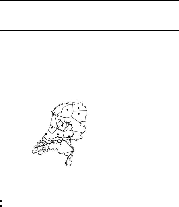
Figure 7.1

The trading areas of the capitals of the twelve provinces in the Netherlands, as predicted by the Voronoi assignment model

147

Chapter 7

VORONOI DIAGRAMS

the cost of transportation to a site equals the Euclidean distance to the site times a fixed price per unit distance;

consumers try to minimize the cost of acquiring the good or service. Usually these assumptions are not completely satisfied: goods may be cheaper at some sites than at others, and the transportation cost between two points is probably not linear in the Euclidean distance between them. But the model above can give a rough approximation of the trading areas of the sites. Areas where the behavior of the people differs from that predicted by the model can be subjected to further research, to see what caused the different behavior.

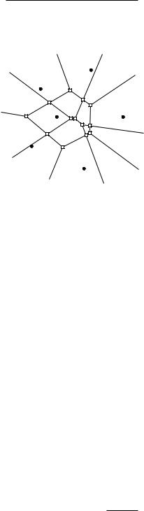
Our interest lies in the geometric interpretation of the model above. The assumptions in the model induce a subdivision of the total area under consideration into regions—the trading areas of the sites—such that the people who live in the same region all go to the same site. Our assumptions imply that people simply get their goods at the nearest site—a fairly realistic situation. This means that the trading area for a given site consists of all those points for which that site is closer than any other site. Figure 7.1 gives an example. The sites in this figure are the capitals of the twelve provinces in the Netherlands.

The model where every point is assigned to the nearest site is called the Voronoi assignment model. The subdivision induced by this model is called the Voronoi diagram of the set of sites. From the Voronoi diagram we can derive all kinds of information about the trading areas of the sites and their relations. For example, if the regions of two sites have a common boundary then these two sites are likely to be in direct competition for customers that live in the boundary region.

The Voronoi diagram is a versatile geometric structure. We have described an application to social geography, but the Voronoi diagram has applications in physics, astronomy, robotics, and many more fields. It is also closely linked to another important geometric structure, the so-called Delaunay triangulation, which we shall encounter in Chapter 9. In the current chapter we shall confine ourselves to the basic properties and the construction of the Voronoi diagram of a set of point sites in the plane.

say that a Voronoi diagram is connected we mean that the union of its edges and vertices forms a connected set. The cell of Vor(P) that corresponds to a site pi is denoted V(pi); we call it the Voronoi cell of pi. (In the terminology of the introduction to this chapter: V(pi) is the trading area of site pi.)

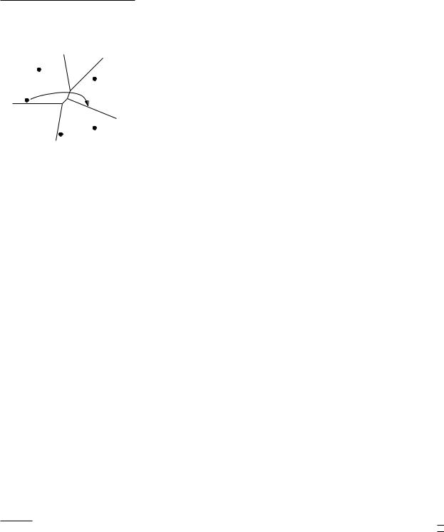
We now take a closer look at the Voronoi diagram. First we study the structure of a single Voronoi cell. For two points p and q in the plane we define the bisector of p and q as the perpendicular bisector of the line segment pq. This bisector splits the plane into two half-planes. We denote the open half-plane that contains p by h(p, q) and the open half-plane that contains q by h(q, p). Notice that r h(p, q) if and only if dist(r, p) < dist(r, q). From this we obtain the following observation.

Observation 7.1 V(pi) = 1 j n, j =i h(pi, p j).

Thus V(pi) is the intersection of n − 1 half-planes and, hence, a (possibly unbounded) open convex polygonal region bounded by at most n −1 vertices and at most n −1 edges.

What does the complete Voronoi diagram look like? We just saw that each cell of the diagram is the intersection of a number of half-planes, so the Voronoi diagram is a planar subdivision whose edges are straight. Some edges are line segments and others are half-lines. Unless all sites are collinear there will be no edges that are full lines:

Theorem 7.2 Let P be a set of n point sites in the plane. If all the sites are collinear then Vor(P) consists of n − 1 parallel lines. Otherwise, Vor(P) is connected and its edges are either segments or half-lines.

Proof. The first part of the theorem is easy to prove, so assume that not all sites in P are collinear.

We first show that the edges of Vor(P) are either segments or half-lines. We already know that the edges of Vor(P) are parts of straight lines, namely parts of the bisectors between pairs of sites. Now suppose for a contradiction that there is an edge e of Vor(P) that is a full line. Let e be on the boundary of the Voronoi cells V(pi) and V(p j). Let pk P be a point that is not collinear with pi and p j. The bisector of p j and pk is not parallel to e and, hence, it intersects e. But then the part of e that lies in the interior of h(pk, p j) cannot be on the boundary of V(p j), because it is closer to pk than to p j, a contradiction.

It remains to prove that Vor(P) is connected. If this were not the case then there would be a Voronoi cell V(pi) splitting the plane into two. Because Voronoi cells are convex, V(pi) would consist of a strip bounded by two parallel full lines. But we just proved that the edges of the Voronoi diagram cannot be full lines, a contradiction.

Now that we understand the structure of the Voronoi diagram we investigate its complexity, that is, the total number of its vertices and edges. Since there are n sites and each Voronoi cell has at most n −1 vertices and edges, the complexity of Vor(P) is at most quadratic. It is not clear, however, whether Vor(P) can actually have quadratic complexity: it is easy to construct an example where a single Voronoi cell has linear complexity, but can it happen that many cells

Section 7.1

DEFINITION AND BASIC PROPERTIES

e pk

149

Chapter 7

VORONOI DIAGRAMS

v∞

CP(q)

q

150

have linear complexity? The following theorem shows that this is not the case and that the average number of vertices of the Voronoi cells is less than six.

Theorem 7.3 For n 3, the number of vertices in the Voronoi diagram of a set of n point sites in the plane is at most 2n −5 and the number of edges is at most

3n −6.

Proof. If the sites are all collinear then the theorem immediately follows from Theorem 7.2, so assume this is not the case. We prove the theorem using Euler’s formula, which states that for any connected planar embedded graph with mv nodes, me arcs, and m f faces the following relation holds:

mv −me + m f = 2.

We cannot apply Euler’s formula directly to Vor(P), because Vor(P) has halfinfinite edges and is therefore not a proper graph. To remedy the situation we add one extra vertex v∞ “at infinity” to the set of vertices and we connect all half-infinite edges of Vor(P) to this vertex. We now have a connected planar graph to which we can apply Euler’s formula. We obtain the following relation between nv, the number of vertices of Vor(P), ne, the number of edges of Vor(P), and n, the number of sites:

Moreover, every edge in the augmented graph has exactly two vertices, so if we sum the degrees of all vertices we get twice the number of edges. Because every vertex, including v∞, has degree at least three we get

Together with equation (7.1) this implies the theorem.

We close this section with a characterization of the edges and vertices of the Voronoi diagram. We know that the edges are parts of bisectors of pairs of sites and that the vertices are intersection points between these bisectors. There is a quadratic number of bisectors, whereas the complexity of the Vor(P) is only linear. Hence, not all bisectors define edges of Vor(P) and not all intersections are vertices of Vor(P). To characterize which bisectors and intersections define features of the Voronoi diagram we make the following definition. For a point q we define the largest empty circle of q with respect to P, denoted by CP(q), as the largest circle with q as its center that does not contain any site of P in its interior. The following theorem characterizes the vertices and edges of the Voronoi diagram.

Theorem 7.4 For the Voronoi diagram Vor(P) of a set of points P the following holds:

(i)A point q is a vertex of Vor(P) if and only if its largest empty circle CP(q)

contains three or more sites on its boundary.

(ii) The bisector between sites pi and p j defines an edge of Vor(P) if and only if there is a point q on the bisector such that CP(q) contains both pi and p j on its boundary but no other site.

Proof. (i) Suppose there is a point q such that CP(q) contains three or more sites on its boundary. Let pi, p j, and pk be three of those sites. Since the interior of CP(q) is empty q must be on the boundary of each of V(pi), V(p j), and V(pk), and q must be a vertex of Vor(P).

On the other hand, every vertex q of Vor(P) is incident to at least three edges and, hence, to at least three Voronoi cells V(pi), V(p j), and V(pk). Vertex q must be equidistant to pi, p j, and pk and there cannot be another site closer to q, since otherwise V(pi), V(p j), and V(pk) would not meet at q. Hence, the interior of the circle with pi, p j, and pk on its boundary does not contain any site.

(ii) Suppose there is a point q with the property stated in the theorem. Since CP(q) does not contain any sites in its interior and pi and p j are on its boundary, we have dist(q, pi) = dist(q, p j) dist(q, pk) for all 1 k n. It follows that q lies on an edge or vertex of Vor(P). The first part of the theorem implies that q cannot be a vertex of Vor(P). Hence, q lies on an edge of Vor(P), which is defined by the bisector of pi and p j.

Conversely, let the bisector of pi and p j define a Voronoi edge. The largest empty circle of any point q in the interior of this edge must contain pi and p j on its boundary and no other sites.

Section 7.2

COMPUTING THE VORONOI DIAGRAM

What happens to the Voronoi diagram at a site event? Recall that the breakpoints on the beach line trace out the edges of the Voronoi diagram. At a site event two new breakpoints appear, which start tracing out edges. In fact, the new breakpoints coincide at first, and then move in opposite directions to trace out the same edge. Initially, this edge is not connected to the rest of the Voronoi diagram above the sweep line. Later on—we will see shortly exactly when this will happen—the growing edge will run into another edge, and it becomes connected to the rest of the diagram.

So now we understand what happens at a site event: a new arc appears on the beach line, and a new edge of the Voronoi diagram starts to be traced out. Is it possible that a new arc appears on the beach line in any other way? The answer is no:

Lemma 7.6 The only way in which a new arc can appear on the beach line is through a site event.

Proof. Suppose for a contradiction that an already existing parabola β j defined by a site p j breaks through the beach line. There are two ways in which this could happen.

The first possibility is that β j breaks through in the middle of an arc of a parabola βi. The moment this is about to happen, βi and β j are tangent, that is, they have exactly one point of intersection. Let y denote the y-coordinate of the sweep line at the moment of tangency. If p j := (p j,x, p j,y), then the parabola β j is given by

The formula for βi is similar, of course. Using that both p j,y and pi,y are larger than y, it is easy to show that it is impossible that βi and β j have only one point of intersection. Hence, a parabola β j never breaks through in the middle of an arc of another parabola βi.

The second possibility is that β j appears in between two arcs. Let these arcs be part of parabolas βi and βk. Let q be the intersection point of βi and βk at which β j is about to appear on the beach line, and assume that βi is on the beach line left of q and βk is on the beach line right of q, as in Figure 7.3. Then there is a circle C that passes through pi, p j, and pk, the sites defining the parabolas. This circle is also tangent to the sweep line . The cyclic order

Figure 7.2

A new arc appears on the beach line because a site is encountered

β j

β j

153

Chapter 7

VORONOI DIAGRAMS

on C, starting at the point of tangency with and going clockwise, is pi, p j, pk, because β j is assumed to appear in between the arcs of βi and βk. Consider an infinitesimal motion of the sweep line downward while keeping the circle C tangent to ; see Figure 7.3. Then C cannot have empty interior and still pass

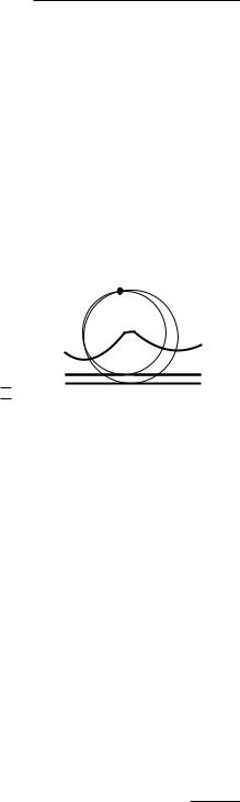
Figure 7.4

An arc disappears from the beach line

through p j: either pi or pk will penetrate the interior. Therefore, in a sufficiently small neighborhood of q the parabola β j cannot appear on the beach line when the sweep line moves downward, because either pi or pk will be closer to than p j.

An immediate consequence of the lemma is that the beach line consists of at most 2n −1 parabolic arcs: each site encountered gives rise to one new arc and the splitting of at most one existing arc into two, and there is no other way an arc can appear on the beach line.

on . There cannot be a site in the interior of this circle: such a site would be closer to q than q is to , contradicting the fact that q is on the beach line. It follows that the point q is a vertex of the Voronoi diagram. This is not very surprising, since we observed earlier that the breakpoints on the beach line trace out the Voronoi diagram. So when an arc disappears from the beach line and two breakpoints meet, two edges of the Voronoi diagram meet as well. We call the event where the sweep line reaches the lowest point of a circle through three sites defining consecutive arcs on the beach line a circle event. From the above we can conclude the following lemma.

Lemma 7.7 The only way in which an existing arc can disappear from the beach line is through a circle event.

Now we know where and how the combinatorial structure of the beach line changes: at a site event a new arc appears, and at a circle event an existing arc drops out. We also know how this relates to the Voronoi diagram under construction: at a site event a new edge starts to grow, and at a circle event two growing edges meet to form a vertex. It remains to find the right data structures to maintain the necessary information during the sweep. Our goal is to compute the Voronoi diagram, so we need a data structure that stores the part of the Voronoi diagram computed thus far. We also need the two ‘standard’ data structures for any sweep line algorithm: an event queue and a structure that represents the status of the sweep line. Here the latter structure is a representation of the beach line. These data structures are implemented in the following way.

We store the Voronoi diagram under construction in our usual data structure for subdivisions, the doubly-connected edge list. A Voronoi diagram, however, is not a true subdivision as defined in Chapter 2: it has edges that are half-lines or full lines, and these cannot be represented in a doublyconnected edge list. During the construction this is not a problem, because the representation of the beach line—described next—will make it possible to access the relevant parts of the doubly-connected edge list efficiently during its construction. But after the computation is finished we want to have a valid doubly-connected edge list. To this end we add a big bounding box to our scene, which is large enough so that it contains all vertices of the Voronoi diagram. The final subdivision we compute will then be the bounding box plus the part of the Voronoi diagram inside it.

The beach line is represented by a balanced binary search tree T; it is the status structure. Its leaves correspond to the arcs of the beach line—which is x-monotone—in an ordered manner: the leftmost leaf represents the leftmost arc, the next leaf represents the second leftmost arc, and so on. Each leaf µ stores the site that defines the arc it represents. The internal nodes of T represent the breakpoints on the beach line. A breakpoint is stored at an internal node by an ordered tuple of sites pi, p j , where pi defines the parabola left of the breakpoint and p j defines the parabola to the right. Using this representation of the beach line, we can find in O(log n)

Section 7.2

COMPUTING THE VORONOI DIAGRAM

155

Chapter 7

VORONOI DIAGRAMS

156

time the arc of the beach line lying above a new site. At an internal node, we simply compare the x-coordinate of the new site with the x-coordinate of the breakpoint, which can be computed from the tuple of sites and the position of the sweep line in constant time. Note that we do not explicitly store the parabolas.

In T we also store pointers to the other two data structures used during the sweep. Each leaf of T, representing an arc α , stores one pointer to a node in the event queue, namely, the node that represents the circle event in which α will disappear. This pointer is nil if no circle event exists where α will disappear, or this circle event hasn’t been detected yet. Finally, every internal node ν has a pointer to a half-edge in the doubly-connected edge list of the Voronoi diagram. More precisely, ν has a pointer to one of the half-edges of the edge being traced out by the breakpoint represented by ν .

The event queue Q is implemented as a priority queue, where the priority of an event is its y-coordinate. It stores the upcoming events that are already known. For a site event we simply store the site itself. For a circle event the event point that we store is the lowest point of the circle, with a pointer to the leaf in T that represents the arc that will disappear in the event.

All the site events are known in advance, but the circle events are not. This brings us to one final issue that we must discuss, namely the detection of circle events.

During the sweep the beach line changes its topological structure at every event. This may cause new triples of consecutive arcs to appear on the beach line and it may cause existing triples to disappear. Our algorithm will make sure that for every three consecutive arcs on the beach line that define a potential circle event, the potential event is stored in the event queue Q. There are two subtleties involved in this. First of all, there can be consecutive triples whose two breakpoints do not converge, that is, the directions in which they move are such that they will not meet in the future; this happens when the breakpoints move along two bisectors away from the intersection point. In this case the triple does not define a potential circle event. Secondly, even if a triple has converging breakpoints, the corresponding circle event need not take place: it can happen that the triple disappears (for instance due to the appearance of a new site on the beach line) before the event has taken place. In this case we call the event a false alarm.

So what the algorithm does is this. At every event, it checks all the new triples of consecutive arcs that appear. For instance, at a site event we can get three new triples: one where the new arc is the left arc of the triple, one where it is the middle arc, and one where it is the right arc. When such a new triple has converging breakpoints, the event is inserted into the event queue Q. Observe that in the case of a site event, the triple with the new arc being the middle one can never cause a circle event, because the left and right arc of the triple come from the same parabola and therefore the breakpoints must diverge. Furthermore, for all disappearing triples it is checked whether they have a corresponding event in Q. If so, the event is apparently a false alarm, and

it is deleted from Q. This can easily be done using the pointers we have from the leaves in T to the corresponding circle events in Q.

Lemma 7.8 Every Voronoi vertex is detected by means of a circle event.

Proof. For a Voronoi vertex q, let pi, p j, and pk be the three sites through which a circle C(pi, p j, pk) passes with no sites in the interior. By Theorem 7.4, such a circle and three sites indeed exist. For simplicity we only prove the case where no other sites lie on C(pi, p j, pk), and the lowest point of C(pi, p j, pk) is not one of the defining sites. Assume without loss of generality that from the lowest point of C(pi, p j, pk), the clockwise traversal of C(pi, p j, pk) encounters the sites pi, p j, pk in this order.

We must show that just before the sweep line reaches the lowest point of C(pi, p j, pk), there are three consecutive arcs α , α and α on the beach line defined by the sites pi, p j, and pk. Only then will the circle event take place. Consider the sweep line an infinitesimal amount before it reaches the lowest point of C(pi, p j, pk). Since C(pi, p j, pk) doesn’t contain any other sites inside or on it, there exists a circle through pi and p j that is tangent to the sweep line, and doesn’t contain sites in the interior. So there are adjacent arcs on the beach line defined by pi and p j. Similarly, there are adjacent arcs on the beach line defined by p j and pk. It is easy to see that the two arcs defined by p j are actually the same arc, and it follows that there are three consecutive arcs on the beach line defined by pi, p j, and pk. Therefore, the corresponding circle event is in Q just before the event takes place, and the Voronoi vertex is detected.

We can now describe the plane sweep algorithm in detail. Notice that after all events have been handled and the event queue Q is empty, the beach line hasn’t disappeared yet. The breakpoints that are still present correspond to the half-infinite edges of the Voronoi diagram. As stated earlier, a doubly-connected edge list cannot represent half-infinite edges, so we must add a bounding box to the scene to which these edges can be attached. The overall structure of the algorithm is as follows.

Algorithm VORONOIDIAGRAM(P)

Input. A set P := {p1, . . . , pn} of point sites in the plane.

Output. The Voronoi diagram Vor(P) given inside a bounding box in a doublyconnected edge list D.

1.Initialize the event queue Q with all site events, initialize an empty status structure T and an empty doubly-connected edge list D.

2.while Q is not empty

3.do Remove the event with largest y-coordinate from Q.

4.if the event is a site event, occurring at site pi

5.then HANDLESITEEVENT(pi)

6.else HANDLECIRCLEEVENT(γ ), where γ is the leaf of T repre-

senting the arc that will disappear

7.The internal nodes still present in T correspond to the half-infinite edges of the Voronoi diagram. Compute a bounding box that contains all vertices of the Voronoi diagram in its interior, and attach the half-infinite edges to the bounding box by updating the doubly-connected edge list appropriately.

Section 7.2

COMPUTING THE VORONOI DIAGRAM

p j C(pi, p j , pk)

pk

pi

157

Chapter 7

VORONOI DIAGRAMS

158

8.Traverse the half-edges of the doubly-connected edge list to add the cell records and the pointers to and from them.

The procedures to handle the events are defined as follows.

HANDLESITEEVENT(pi)

1.If T is empty, insert pi into it (so that T consists of a single leaf storing pi) and return. Otherwise, continue with steps 2– 5.

2.Search in T for the arc α vertically above pi. If the leaf representing α has a pointer to a circle event in Q, then this circle event is a false alarm and it must be deleted from Q.

3.Replace the leaf of T that represents α with a subtree having three leaves.

The middle leaf stores the new site pi and the other two leaves store the site p j that was originally stored with α . Store the tuples p j, pi and pi, p j representing the new breakpoints at the two new internal nodes. Perform rebalancing operations on T if necessary.

4.Create new half-edge records in the Voronoi diagram structure for the edge separating V(pi) and V(p j), which will be traced out by the two new breakpoints.

5.Check the triple of consecutive arcs where the new arc for pi is the left arc to see if the breakpoints converge. If so, insert the circle event into Q and add pointers between the node in T and the node in Q. Do the same for the triple where the new arc is the right arc.

HANDLECIRCLEEVENT(γ )

1.Delete the leaf γ that represents the disappearing arc α from T. Update the tuples representing the breakpoints at the internal nodes. Perform

rebalancing operations on T if necessary. Delete all circle events involving α from Q; these can be found using the pointers from the predecessor and the successor of γ in T. (The circle event where α is the middle arc is currently being handled, and has already been deleted from Q.)

2.Add the center of the circle causing the event as a vertex record to the doubly-connected edge list D storing the Voronoi diagram under construction. Create two half-edge records corresponding to the new breakpoint of the beach line. Set the pointers between them appropriately. Attach the three new records to the half-edge records that end at the vertex.

3.Check the new triple of consecutive arcs that has the former left neighbor of α as its middle arc to see if the two breakpoints of the triple converge. If so, insert the corresponding circle event into Q. and set pointers between the new circle event in Q and the corresponding leaf of T. Do the same for the triple where the former right neighbor is the middle arc.

Lemma 7.9 The algorithm runs in O(n log n) time and it uses O(n) storage.

Proof. The primitive operations on the tree T and the event queue Q, such as inserting or deleting an element, take O(log n) time each. The primitive operations on the doubly-connected edge list take constant time. To handle an event we do a constant number of such primitive operations, so we spend

O(log n) time to process an event. Obviously, there are n site events. As for the number of circle events, we observe that every such event that is processed defines a vertex of Vor(P). Note that false alarms are deleted from Q before they are processed. They are created and deleted while processing another, real event, and the time we spend on them is subsumed under the time we spend to process this event. Hence, the number of circle events that we process is at most 2n −5. The time and storage bounds follow.

Before we state the final result of this section we should say a few words about degenerate cases.

The algorithm handles the events from top to bottom, so there is a degeneracy when two or more events lie on a common horizontal line. This happens, for example, when there are two sites with the same y-coordinate. These events can be handled in any order when their x-coordinates are distinct, so we can break ties between events with the same y-coordinate but with different x-coordinates arbitrarily. However, if this happens right at the start of the algorithm, that is, if the second site event has the same y-coordinate as the first site event, then special code is needed because there is no arc above the second site yet. Now suppose there are event points that coincide. For instance, there will be several coincident circle events when there are four or more co-circular sites, such that the interior of the circle through them is empty. The center of this circle is a vertex of the Voronoi diagram. The degree of this vertex is at least four. We could write special code to handle such degenerate cases, but there is no need to do so. What will happen if we let the algorithm handle these events in arbitrary order? Instead of producing a vertex with degree four, it will just produce two vertices with degree three at the same location, with a zero length edge between them. These degenerate edges can be removed in a post-processing step, if required.

Besides these degeneracies in choosing the order of the events we may also encounter degeneracies while handling an event. This occurs when a site pi that we process happens to be located exactly below the breakpoint between two arcs on the beach line. In this case the algorithm splits either of these two arcs and inserts the arc for pi in between the two pieces, one of which has zero length. This piece of zero length now is the middle arc of a triple that defines a circle event. The lowest point of this circle coincides with pi. The algorithm inserts this circle event into the event queue Q, because there are three consecutive arcs on the beach line that define it. When this circle event is handled, a vertex of the Voronoi diagram is correctly created and the zero length arc can be deleted later. Another degeneracy occurs when three consecutive arcs on the beach line are defined by three collinear sites. Then these sites don’t define a circle, nor a circle event.

We conclude that the above algorithm handles degenerate cases correctly.

Theorem 7.10 The Voronoi diagram of a set of n point sites in the plane can be computed with a sweep line algorithm in O(n log n) time using O(n) storage.

Section 7.2

COMPUTING THE VORONOI DIAGRAM

zero-length edge

159

Chapter 7

VORONOI DIAGRAMS

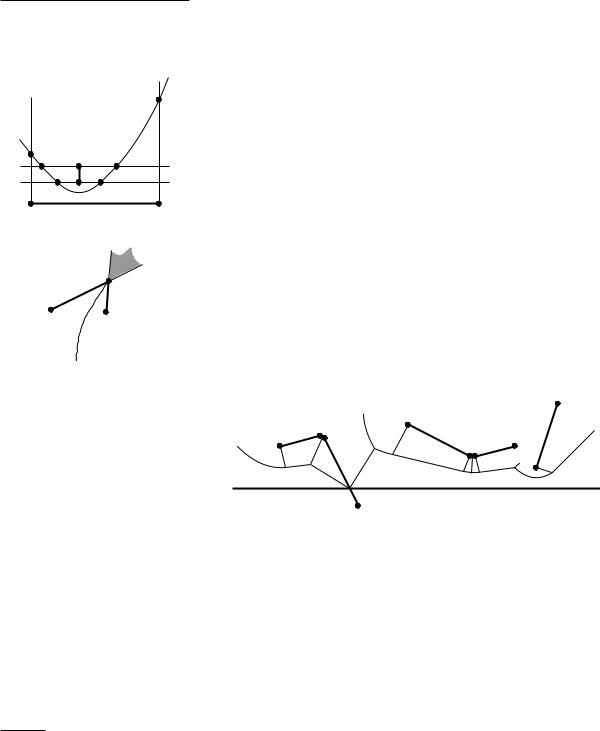
Figure 7.5

The beach line for a set of line segment sites. The breakpoints trace the dashed arcs, which include the Voronoi edges

160

7.3Voronoi Diagrams of Line Segments

The Voronoi diagram can also be defined for objects other than points. The distance from a point in the plane to an object is then measured to the closest point on the object. Whereas the bisector of two points is simply a line, the bisector of two disjoint line segments has a more complex shape. It consists of up to seven parts, where each part is either a line segment or a parabolic arc. Parabolic arcs occur if the closest point of one line segment is an endpoint and the closest point of the other line segment is in its interior. In all other cases the bisector part is straight. Although bisectors and therefore the Voronoi diagram are somewhat more complex, the number of vertices, edges, and faces in the Voronoi diagram of n disjoint line segments is still only O(n).

Assume for a moment that we allow the line segments to be non-crossing, that is, we allow them to share endpoints. Then a whole region of the plane can be equally close to two line segments via their common endpoint, and bisectors are not even curves anymore. To avoid the complications that arise in defining and computing Voronoi diagrams of line segments that share endpoints, we will simply assume here that all line segments are strictly disjoint. In many applications we can simply shorten the line segments very slightly to obtain disjoint line segments.

The sweep line algorithm for points can be adapted to the case of line segment sites. Let S = {s1, . . . , sn} be a set of n disjoint line segments. We call the segments of S sites as before, and use the terms site endpoint and site interior in the following description.

Recall that our algorithm for point sites maintained a beach line: a piecewise parabolic x-monotone curve such that, for points on the curve, the distance to the closest site above the sweep line is equal to the distance to the sweep line. What does the beach line look like when the sites are segments? First we note that a line segment site may be partially above and partially below the sweep line. When defining the beach line, we consider only those parts of the sites that are above the sweep line. Hence, for a given position of the sweep line , the beach line consists of those points such that the distance to the closest portion of a site above is equal to the distance to . This means that the beach line now consists of parabolic arcs and straight line segments. A parabolic arc arises when that part of the beach line is closest to a site endpoint, and a straight line segment arises when that part of the beach line is closest to a site interior. Note that if a site interior intersects , then the beach line will have two straight line segments ending at the intersection—see site s2 in Figure 7.5.

The breakpoints between parabolic arcs and straight segments on the beach line arise in several different ways. Figure 7.5 illustrates this. Assume any position of the sweep line during the downward sweep to analyze the types of breakpoint:

If a point p is closest to two site endpoints while being equidistant from them and , then p is a breakpoint that traces a line segment (as in the point site case).

If a point p is closest to two site interiors while being equidistant from them and , then p is a breakpoint that traces a line segment.

If a point p is closest to a site endpoint and a site interior of different sites while being equidistant from them and , then p is a breakpoint that traces a parabolic arc.

If a point p is closest to a site endpoint, the shortest distance is realized by a segment that is perpendicular to the line segment site, and p has the same distance from , then p is a breakpoint that traces a line segment.

If a site interior intersects the sweep line, then the intersection is a breakpoint that traces a line segment (the site interior).

In the fourth and fifth cases, the breakpoint does not actually trace an arc of the Voronoi diagram, because only one site is involved. For the proper operation of the algorithm, dealing with such breakpoints and corresponding events is still necessary.

As in the sweep line algorithm for point sites, we again have site events and circle events. A site event occurs when the sweep line reaches a site endpoint. Obviously, site events at upper endpoints should be handled differently from site events at lower endpoints. At an upper endpoint, an arc of the beach line is split into two, and in between, four new arcs appear. The breakpoints between these four arcs are of the last two types. At a lower endpoint, the breakpoint that is the intersection of the site interior with the sweep line is replaced by two breakpoints of the fourth type, with a parabolic arc in between (for the newly discovered site endpoint).

Similarly, there are several types of circle event. They all correspond to the disappearance of an arc of the beach line, and they occur when the sweep line reaches the bottom of an empty circle that is defined by two or three sites above the sweep line. The centers of these empty circles are at locations where two consecutive breakpoints will meet. Depending on the types of the breakpoints that meet, several different cases can be distinguished and handled. If the two breakpoints are of any of the first three types, then three sites are involved. If one of the breakpoints is of the fourth type, then only two sites are involved. Breakpoints of the fifth type cannot be involved for disjoint line segments.

Notice that the Voronoi diagram that the algorithm computes is a subdivision with straight edges and parabolic arcs. Can we store this type of subdivision in a doubly-connected edge list? This is indeed possible, and the structure need not even be adapted. With each face, we store the corresponding site, so for any

Section 7.3

VORONOI DIAGRAMS OF LINE

SEGMENTS

161

Chapter 7

VORONOI DIAGRAMS

half-edge e we can determine the two sites that have e on their bisector (using IncidentFace(e) and IncidentFace(Twin(e))). Since we can also easily find the two vertices between which the edge lies (Origin(e) and Origin(Twin(e))), we can determine the shape of any edge in constant time.

The whole sweep line algorithm is now just an extension of the one for point sites, with more cases to be distinguished and handled. However, the algorithm still has only O(n) events, and each can be handled in O(log n) time.

Theorem 7.11 The Voronoi diagram of a set of n disjoint line segment sites can be computed in O(n log n) time using O(n) storage.

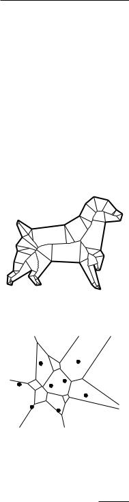
One of the applications of the Voronoi diagram for line segments is in motion planning (covered more extensively in Chapter 13). Assume that a set of obstacles is given, consisting of n line segments in total, and that we have a robot R. We assume that the robot can move freely in all directions, and is approximated well by an enclosing disc D. Suppose that we wish to find a collision-free motion from one location of the robot to another, or to decide that none exists.

One motion-planning technique is called retraction. The idea of retraction is that the arcs of the Voronoi diagram define the middle between the line segments, and therefore define a path with the most clearance. So a path over the arcs of the Voronoi diagram is the best option for a collision-free path. Figure 7.6 shows a set of line segments inside a rectangle, together with a Voronoi diagram of the line segments and the sides of the rectangle.

Algorithm RETRACTION(S, qstart, qend, r)

Input. A set S := {s1, . . . , sn} of disjoint line segments in the plane, and two discs Dstart and Dend centered at qstart and qend with radius r. The two disc positions do not intersect any line segment of S.

Output. A path that connects qstart to qend such that no disc of radius r with its center on the path intersects any line segment of S. If no such path exists, this is reported.

1.Compute the Voronoi diagram Vor(S) of S inside a sufficiently large bounding box.

2.Locate the cells of Vor(P) that contain qstart and qend.

3.Determine the point pstart on Vor(S) by moving qstart away from the nearest line segment in S. Similarly, determine the point pend on Vor(S) by moving

qend away from the nearest line segment in S. Add pstart and pend as vertices to Vor(S), splitting the arcs on which they lie into two.

4.Let G be the graph corresponding to the vertices and edges of the Voronoi diagram. Remove all edges from G for which the smallest distance to the nearest sites is smaller than or equal to r.

5.Determine with depth-first search whether a path exists from pstart to pend in G. If so, report the line segment from qstart to pstart, the path in G from pstart to pend, and the line segment from pend to qend as the path. Otherwise, report that no path exists.

The line segment connecting qstart to pstart cannot give a collision, because the disc only moves further away from the nearest obstacle. Similarly, the line segment between pend and qend is collision-free. For any two discs centered on the Voronoi diagram, a collision-free path between them exists on the Voronoi diagram if and only if such a path exists at all. Hence, for a disc-shaped robot, a path is found if one exists.

Theorem 7.12 Given n disjoint line segment obstacles and a disc-shaped robot, the existence of a collision-free path between two positions of the robot can be determined in O(n log n) time using O(n) storage.

Section 7.4

FARTHEST-POINT VORONOI

DIAGRAMS

Chapter 7

VORONOI DIAGRAMS

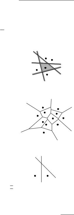
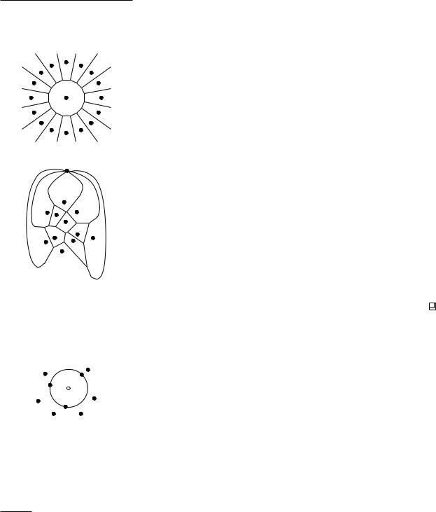
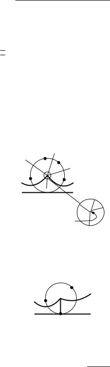
Clearly, there must be at least one point on Couter, otherwise we can reduce the size of Couter, and at least one point on Cinner, otherwise we can increase the size of Cinner. But one point on each bounding circle cannot give us a smallest-width annulus yet. There appear to be three different cases, each with a total of four points on the two circles (Figure 7.7):

Couter contains at least three points of P, and Cinner contains at least one point of P.

Couter contains at least one point of P, and Cinner contains at least three points of P.

Couter and Cinner both contain two points of P.

Figure 7.7

Three cases of the smallest-width annulus

cell of p j

p j

164

If Cinner or Couter contains fewer points than listed in any of these cases, then we can always find an annulus with a smaller width. The problem of finding the smallest-width annulus enclosing a given point set looks similar to the problem of finding the smallest disc enclosing a point set, studied in Section 4.7. The technique we used for the smallest-disc problem, however, does not work for the smallest-width annulus: the property that an added point that does not lie in the optimal annulus so far must always lie on the boundary of the new optimal annulus does not hold.

Finding the smallest-width annulus is equivalent to finding its center point. Once the center point—let’s call it q—is fixed, the annulus is determined by the points of P that are closest to and farthest from q. If we have the Voronoi diagram of P, then the closest point is the one in whose cell q lies. It turns out that a similar structure exists for the farthest point, namely the farthest-point Voronoi diagram. This divides the plane into cells in which the same point of P is the farthest point. The farthest-point Voronoi cell of a point pi is the intersection of n −1 half-planes, just as for a standard Voronoi cell, but we take the “other sides” of the bisectors, the sides where pi is farther away. Hence, all cells of the farthest-point Voronoi diagram are convex. Not every point of P has a cell in the farthest-point Voronoi diagram: the intersections of the half-planes can be empty. It is not hard to see that for any point in the plane, its farthest point in the set P must be a point that lies on the convex hull of P. Therefore, a point that lies inside the convex hull cannot have a cell in the farthest-point Voronoi diagram.

Observation 7.13 Given a set P of points in the plane, a point of P has a cell in the farthest-point Voronoi diagram if and only if it is a vertex of the convex hull of P.

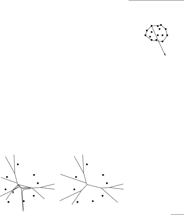
We can prove more properties of the farthest-point Voronoi diagram. Suppose that a point pi P lies on the convex hull, and let q be some point in the plane for which pi is the farthest point. Let (pi, q) be the line through pi and q. Then all points on the half-line starting at q, contained in (pi, q), and not containing pi, must also be in the farthest-point Voronoi cell of pi. This implies that all cells are unbounded. The vertices and edges of the farthest-point Voronoi diagram form a tree-like structure (in the graph sense), because the diagram is connected and does not have cycles. A cycle would imply a bounded cell.

We can show that the farthest-point Voronoi diagram of n points has O(n) vertices, edges, and cells (see also Exercise 7.14). There is another interesting property: the center of the smallest enclosing disc (see Section 4.7) is either a vertex of the farthest-point Voronoi diagram or the midpoint of two sites defining an edge of the farthest-point Voronoi diagram. In the former case, there are three equidistant farthest points, and in the latter case, two. Clearly, the center of the smallest enclosing disc cannot have just one point that is farthest from it.

Since the farthest-point Voronoi diagram has half-infinite edges, we cannot store it in a doubly-connected edge list, but we can adapt the structure slightly to deal with such subdivisions. We use a special vertex-like record as the origin of each half-edge that has no real vertex as its origin. These new records store the direction of the half-infinite edge instead of coordinates. Furthermore, halfedge records corresonding to half-infinite edges have either Next(e) or Prev(e) undefined. We shall still use the term “doubly-connected edge list” for this adapted version.

We now present an algorithm to compute the farthest-point Voronoi diagram of a set P of n points in the plane. First, we compute the convex hull of P, take its vertices, and put them in random order. Let this random order be p1, . . . , ph. We remove the points ph, . . . , p4 one by one from the cyclic order, and when removing pi, store its clockwise neighbor cw(pi) and counterclockwise neighbor ccw(pi) at the time of removal. After a point has been removed, it cannot be the clockwise or counterclockwise neighbor anymore of points removed later.

Section 7.4

FARTHEST-POINT VORONOI

DIAGRAMS

pi

q

Chapter 7

VORONOI DIAGRAMS

cell of p j

p j

166

the incremental construction. Then we insert the remaining points p4, . . . , ph while constructing the farthest-point Voronoi diagram. To be able to add the farthest-point Voronoi cell of pi efficiently, given the farthest-point Voronoi diagram of {p1, . . . , pi−1}, we maintain a pointer for each point p j, 1 j < i, to the half-infinite half-edge of the doubly-connected edge list that is most counterclockwise in a traversal of the boundary of the farthest-point Voronoi cell of p j.

We now look at the addition of the cell of pi in more detail, see Figure 7.8. The cell will come “in between” the cells of cw(pi) and ccw(pi). Just before pi is added, cw(pi) and ccw(pi) are each other’s neighbors on the convex hull of {p1, . . . , pi−1}, so their cells are separated by a half-infinite edge that is part of their bisector. The point ccw(pi) has a pointer to this edge. The bisector of pi and ccw(pi) will give a new half-infinite edge that lies in the farthestpoint Voronoi cell of ccw(pi), and is part of the boundary of the farthest-point Voronoi cell of pi. We traverse the cell of ccw(pi) in the clockwise direction to see which edge the bisector intersects. On the other side of this edge is the farthest-point Voronoi cell of another point p j from {p1, . . . , pi−1}, and the bisector of p j and pi will also give an edge of the farthest-point Voronoi cell of pi. We again traverse the cell of p j in the clockwise direction to determine where the other insertion of the cell boundary and the bisector is located. By tracing cell boundaries in clockwise order, we trace the farthest-point Voronoi cell in counterclockwise order. The last bisector that we will find is with cw(pi), and it will give a new half-infinite edge in the farthest-point Voronoi diagram. All new edges found are added to the doubly-connected edge list representation, after which all edges that lie inside the farthest-point Voronoi cell of pi are removed. They are no longer valid edges of the farthest-point Voronoi diagram of {p1, . . . , pi}.

In short, the insertion of the next farthest-point Voronoi cell is done by tracing the new cell with the help of the existing diagram, adding the new edges, and removing the edges that have become obsolete.

Theorem 7.14 Given a set of n points in the plane, its farthest-point Voronoi diagram can be computed in O(n log n) expected time using O(n) storage.

Proof. It takes O(n log n) time to compute the h points on the convex hull in counterclockwise order. The farthest-point Voronoi diagram actually takes only O(h) expected time to construct after we have the points on the convex hull in sorted order. To see this, we apply backwards analysis. We consider the situation after the insertion of the cell of pi. We observe that if the cell of pi has k edges on its boundary, then the traversal performed to trace this cell visited k cells in the farthest-point Voronoi diagram of {p1, . . . , pi−1}, and visited at most 4k −6 boundary edges of these cells in total.

The farthest-point Voronoi diagram of {p1, . . . , pi} has at most 2i −3 edges (see Exercise 7.14), each used by two cells. Since every point of {p1, . . . , pi} has the same probability of having been the last one added, the expected size of the cell of pi is less than four. Hence, the expected time needed for each insertion is O(1), and the algorithm runs in O(h) expected time.

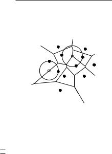
Now we return to the problem of computing the smallest-width annulus. Suppose that the smallest-width annulus is such that Cinner contains at least three points of P. Then its center is a vertex of the normal Voronoi diagram of P. Similarly, if the smallest-width annulus is such that Couter contains at least three points of P, its center is a vertex of the farthest-point Voronoi diagram of P. Finally, if the smallest-width annulus is such that Cinner and Couter both contain two points of P, then its center must lie on an edge of the Voronoi diagram and on an edge of the farthest-point Voronoi diagram simultaneously. This means that we can obtain a reasonably small set of points that must contain the center of a smallest-width annulus.

To do this, we generate the vertices of the overlay of the Voronoi diagram and the farthest-point Voronoi diagram. The vertices of the overlay are exactly the candidate centers of the smallest-width annulus, covering all three cases. We don’t really need to compute the overlay itself. Once we know a vertex and the four points that determine Cinner and Couter, we can compute the smallest-width annulus of those four points directly in O(1) time. This is a candidate for the smallest-width annulus.

The whole algorithm to compute the smallest-width annulus of a set P of n points in the plane is as follows. Compute the Voronoi diagram and the farthestpoint Voronoi diagram of P. For each vertex of the farthest-point Voronoi diagram, determine the point of P that is closest. For each vertex of the normal Voronoi diagram, determine the point of P that is farthest. This gives us O(n) sets of four points that define the candidate annuli in the first and second cases. Next, for every pair of edges, one from each of the diagrams, test if they intersect. If so, we have another set of four points that forms a candidate annulus. For all candidates of all three types, choose the one that gives the smallest-width annulus as the solution.

Theorem 7.15 Given a set P of n points in the plane, the smallest-width annulus (and the roundness) can be determined in O(n2) time using O(n) storage.

Section 7.5

NOTES AND COMMENTS

Chapter 7

VORONOI DIAGRAMS

contains an ample treatment of Voronoi diagrams and their applications. We confine ourselves in this section to a discussion of the various aspects of Voronoi diagrams encountered in the computational geometry literature.

In this chapter we have proved some properties of the Voronoi diagram, but it has many more. For example, if one connects all the pairs of sites whose Voronoi cells are adjacent then the resulting set of segments forms a triangulation of the point set, called the Delaunay triangulation. This triangulation, which has some very nice properties, is the topic of Chapter 9.

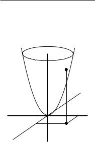
There is a beautiful connection between Voronoi diagrams and convex polyhedra. Consider the transformation that maps a point p = (px, py) in E2 to the non-vertical plane h(p) : z = 2pxx + 2pyy −(p2x + p2y ) in E3. Geometrically, h(p) is the plane that is tangent to the unit paraboloid U : z = x2 + y2 at the point vertically above (px, py, 0). For a set P of point sites in the plane, let H(P) be the set of planes that are the images of the sites in P. Now consider the convex polyhedron P that is the intersection of all positive half-spaces defined by the planes in H(P), that is, P := h H(P) h+, where h+ denotes the half-space above h. Surprisingly, if we project the edges and vertices of the polyhedron vertically downwards onto the xy-plane, we get the Voronoi diagram of P [167]. See Chapter 11 for a more extensive description of this transformation. A similar transformation exists for the farthest-point Voronoi diagram.

Note that the L2-metric is simply the Euclidean metric. There are several papers dealing with Voronoi diagrams in these metrics [118, 248, 252]. One can also define a distance function by assigning a weight to each site. Now the distance from a site to a point is the Euclidean distance to the point, plus its additive weight. The resulting diagrams are called weighted Voronoi diagrams [183]. The weight can also be used to define the distance from a site to a point as the Euclidean distance times the weight. Diagrams based on this multiplicatively weighted distance are also called weighted Voronoi diagrams [29]. Power diagrams [25, 26, 27, 30] are another generalization of Voronoi diagrams where a different distance function is used. It is even possible to drop the distance function altogether and define the Voronoi diagram in terms only of bisectors between pairs of sites. Such diagrams are called abstract Voronoi diagrams [240, 241, 242, 274].

Other generalizations concern the shape of the sites. We have seen the Voronoi diagram of a set of disjoint line segments in this chapter. We discussed the application of this diagram to motion planning using the retraction technique; Chapter 13 discusses motion planning in general.

An important special case of the Voronoi diagram of line segments is the Voronoi diagram of the edges of a simple polygon, interior to the polygon itself. Since the edges share endpoints, there can be whole regions inside the polygon where two edges are equally close. This occurs at every reflex vertex of the polygon. The Voronoi diagram is the subdivision of the interior of the polygon into faces where one or two edges are the closest. This Voronoi diagram is also known as the medial axis or skeleton, and it has applications in shape analysis [366, 377]. The medial axis can be computed in time linear in the number of edges of the polygon [123].

Instead of partitioning the space into regions according to the closest sites, one can also partition it according to the k closest sites, for some 1 k n −1. The diagrams obtained in this way are called higher-order Voronoi diagrams, and, for given k, the diagram is called the order-k Voronoi diagram [6, 31, 70, 98]. Note that the order-1 Voronoi diagram is nothing more than the standard Voronoi diagram. The order-(n − 1) Voronoi diagram is the farthest-point Voronoi diagram, because the Voronoi cell of a point pi is now the region of points for which pi is the farthest site. The maximum complexity of the order-k Voronoi diagram of a set of n point sites in the plane is Θ(k(n − k)) [249]. Currently

the best known algorithms for computing the order-k Voronoi diagram run in O(n log3 n + nk) time [6] and in O(n log n + nk2c log k) time [326], where c is a

constant.

The farthest-point Voronoi diagram takes O(n log n) time to compute, but if the points are in convex position and are given in the order along the convex hull, then there exists a simple O(n) expected-time algorithm [116], given in this chapter, and also an O(n) time deterministic algorithm [11]. Testing the roundness of an object or set of points is a problem that arises in metrology, the science of measurement. Several definitions of roundness exist, the one used in this chapter being the most widely accepted one. A quadratic-time

Section 7.5

NOTES AND COMMENTS

169

Chapter 7

VORONOI DIAGRAMS

algorithm for the roundness problem was given by Ebarra et al. [155]. A complex, subquadratic-time algorithm was suggested by Agarwal and Sharir [9]. In special cases that correspond to point sets that may occur in practice, linear-time or near-linear-time algorithms exist [52, 142, 187]. A survey of computational metrology has been given by Yap and Chang [396].

7.11 Let P be a set of n points in the plane. Give an O(n log n) time algorithm to find for each point p in P another point in P that is closest to it.

7.12Let the Voronoi diagram of a point set P be stored in a doubly-connected edge list inside a bounding box. Give an algorithm to compute all points of P that lie on the boundary of the convex hull of P in time linear in the output size. Assume that your algorithm receives as its input a pointer to the record of some half-edge whose origin lies on the bounding box.

7.13For each of the ten breakpoints shown in Figure 7.5, determine which of the five types it corresponds to.

7.14Show that the farthest point Voronoi diagram on n points in the plane has at most 2n − 3 (bounded or unbounded) edges. Also give an exact bound on the maximum number of vertices in the farthest point Voronoi diagram.

7.15Show that the smallest width annulus cannot be constructed with randomized incremental construction. To this end, show that a point pi can be added to a set Pi−1 that does not lie in the minimum width annulus, but does not lie on the boundary of the smallest width annulus of

Pi := Pi−1 ∩{pi}.

7.16Show that for some set P of n points, there can be Ω(n2) intersections between the edges of the Voronoi diagram and the farthest site Voronoi diagram.

7.17Show that if there are only O(n) intersections between the edges of the

Voronoi diagram and the farthest site Voronoi diagram, then the smallest width annulus can be computed in O(n log n) expected time.

7.18* In the Voronoi assignment model the goods or services that the consumers want to acquire have the same market price at every site. Suppose this is not the case, and that the price of the good at site pi is wi. The trading areas of the sites now correspond to the cells in the weighted Voronoi diagram of the sites (see Section 7.5), where site pi has an additive weight wi. Generalize the sweep line algorithm of Section 7.2 to this case.

7.19* Suppose that we are given a subdivision of the plane into n convex regions. We suspect that this subdivision is a Voronoi diagram, but we do not know the sites. Develop an algorithm that finds a set of n point sites whose Voronoi diagram is exactly the given subdivision, if such a set exists.

Section 7.6

EXERCISES