

- •About the author
- •Brief Contents
- •Contents
- •Preface
- •This Book’s Approach
- •What’s New in the Seventh Edition?
- •The Arrangement of Topics
- •Part One, Introduction
- •Part Two, Classical Theory: The Economy in the Long Run
- •Part Three, Growth Theory: The Economy in the Very Long Run
- •Part Four, Business Cycle Theory: The Economy in the Short Run
- •Part Five, Macroeconomic Policy Debates
- •Part Six, More on the Microeconomics Behind Macroeconomics
- •Epilogue
- •Alternative Routes Through the Text
- •Learning Tools
- •Case Studies
- •FYI Boxes
- •Graphs
- •Mathematical Notes
- •Chapter Summaries
- •Key Concepts
- •Questions for Review
- •Problems and Applications
- •Chapter Appendices
- •Glossary
- •Translations
- •Acknowledgments
- •Supplements and Media
- •For Instructors
- •Instructor’s Resources
- •Solutions Manual
- •Test Bank
- •PowerPoint Slides
- •For Students
- •Student Guide and Workbook
- •Online Offerings
- •EconPortal, Available Spring 2010
- •eBook
- •WebCT
- •BlackBoard
- •Additional Offerings
- •i-clicker
- •The Wall Street Journal Edition
- •Financial Times Edition
- •Dismal Scientist
- •1-1: What Macroeconomists Study
- •1-2: How Economists Think
- •Theory as Model Building
- •The Use of Multiple Models
- •Prices: Flexible Versus Sticky
- •Microeconomic Thinking and Macroeconomic Models
- •1-3: How This Book Proceeds
- •Income, Expenditure, and the Circular Flow
- •Rules for Computing GDP
- •Real GDP Versus Nominal GDP
- •The GDP Deflator
- •Chain-Weighted Measures of Real GDP
- •The Components of Expenditure
- •Other Measures of Income
- •Seasonal Adjustment
- •The Price of a Basket of Goods
- •The CPI Versus the GDP Deflator
- •The Household Survey
- •The Establishment Survey
- •The Factors of Production
- •The Production Function
- •The Supply of Goods and Services
- •3-2: How Is National Income Distributed to the Factors of Production?
- •Factor Prices
- •The Decisions Facing the Competitive Firm
- •The Firm’s Demand for Factors
- •The Division of National Income
- •The Cobb–Douglas Production Function
- •Consumption
- •Investment
- •Government Purchases
- •Changes in Saving: The Effects of Fiscal Policy
- •Changes in Investment Demand
- •3-5: Conclusion
- •4-1: What Is Money?
- •The Functions of Money
- •The Types of Money
- •The Development of Fiat Money
- •How the Quantity of Money Is Controlled
- •How the Quantity of Money Is Measured
- •4-2: The Quantity Theory of Money
- •Transactions and the Quantity Equation
- •From Transactions to Income
- •The Assumption of Constant Velocity
- •Money, Prices, and Inflation
- •4-4: Inflation and Interest Rates
- •Two Interest Rates: Real and Nominal
- •The Fisher Effect
- •Two Real Interest Rates: Ex Ante and Ex Post
- •The Cost of Holding Money
- •Future Money and Current Prices
- •4-6: The Social Costs of Inflation
- •The Layman’s View and the Classical Response
- •The Costs of Expected Inflation
- •The Costs of Unexpected Inflation
- •One Benefit of Inflation
- •4-7: Hyperinflation
- •The Costs of Hyperinflation
- •The Causes of Hyperinflation
- •4-8: Conclusion: The Classical Dichotomy
- •The Role of Net Exports
- •International Capital Flows and the Trade Balance
- •International Flows of Goods and Capital: An Example
- •Capital Mobility and the World Interest Rate
- •Why Assume a Small Open Economy?
- •The Model
- •How Policies Influence the Trade Balance
- •Evaluating Economic Policy
- •Nominal and Real Exchange Rates
- •The Real Exchange Rate and the Trade Balance
- •The Determinants of the Real Exchange Rate
- •How Policies Influence the Real Exchange Rate
- •The Effects of Trade Policies
- •The Special Case of Purchasing-Power Parity
- •Net Capital Outflow
- •The Model
- •Policies in the Large Open Economy
- •Conclusion
- •Causes of Frictional Unemployment
- •Public Policy and Frictional Unemployment
- •Minimum-Wage Laws
- •Unions and Collective Bargaining
- •Efficiency Wages
- •The Duration of Unemployment
- •Trends in Unemployment
- •Transitions Into and Out of the Labor Force
- •6-5: Labor-Market Experience: Europe
- •The Rise in European Unemployment
- •Unemployment Variation Within Europe
- •The Rise of European Leisure
- •6-6: Conclusion
- •7-1: The Accumulation of Capital
- •The Supply and Demand for Goods
- •Growth in the Capital Stock and the Steady State
- •Approaching the Steady State: A Numerical Example
- •How Saving Affects Growth
- •7-2: The Golden Rule Level of Capital
- •Comparing Steady States
- •The Transition to the Golden Rule Steady State
- •7-3: Population Growth
- •The Steady State With Population Growth
- •The Effects of Population Growth
- •Alternative Perspectives on Population Growth
- •7-4: Conclusion
- •The Efficiency of Labor
- •The Steady State With Technological Progress
- •The Effects of Technological Progress
- •Balanced Growth
- •Convergence
- •Factor Accumulation Versus Production Efficiency
- •8-3: Policies to Promote Growth
- •Evaluating the Rate of Saving
- •Changing the Rate of Saving
- •Allocating the Economy’s Investment
- •Establishing the Right Institutions
- •Encouraging Technological Progress
- •The Basic Model
- •A Two-Sector Model
- •The Microeconomics of Research and Development
- •The Process of Creative Destruction
- •8-5: Conclusion
- •Increases in the Factors of Production
- •Technological Progress
- •The Sources of Growth in the United States
- •The Solow Residual in the Short Run
- •9-1: The Facts About the Business Cycle
- •GDP and Its Components
- •Unemployment and Okun’s Law
- •Leading Economic Indicators
- •9-2: Time Horizons in Macroeconomics
- •How the Short Run and Long Run Differ
- •9-3: Aggregate Demand
- •The Quantity Equation as Aggregate Demand
- •Why the Aggregate Demand Curve Slopes Downward
- •Shifts in the Aggregate Demand Curve
- •9-4: Aggregate Supply
- •The Long Run: The Vertical Aggregate Supply Curve
- •From the Short Run to the Long Run
- •9-5: Stabilization Policy
- •Shocks to Aggregate Demand
- •Shocks to Aggregate Supply
- •10-1: The Goods Market and the IS Curve
- •The Keynesian Cross
- •The Interest Rate, Investment, and the IS Curve
- •How Fiscal Policy Shifts the IS Curve
- •10-2: The Money Market and the LM Curve
- •The Theory of Liquidity Preference
- •Income, Money Demand, and the LM Curve
- •How Monetary Policy Shifts the LM Curve
- •Shocks in the IS–LM Model
- •From the IS–LM Model to the Aggregate Demand Curve
- •The IS–LM Model in the Short Run and Long Run
- •11-3: The Great Depression
- •The Spending Hypothesis: Shocks to the IS Curve
- •The Money Hypothesis: A Shock to the LM Curve
- •Could the Depression Happen Again?
- •11-4: Conclusion
- •12-1: The Mundell–Fleming Model
- •The Goods Market and the IS* Curve
- •The Money Market and the LM* Curve
- •Putting the Pieces Together
- •Fiscal Policy
- •Monetary Policy
- •Trade Policy
- •How a Fixed-Exchange-Rate System Works
- •Fiscal Policy
- •Monetary Policy
- •Trade Policy
- •Policy in the Mundell–Fleming Model: A Summary
- •12-4: Interest Rate Differentials
- •Country Risk and Exchange-Rate Expectations
- •Differentials in the Mundell–Fleming Model
- •Pros and Cons of Different Exchange-Rate Systems
- •The Impossible Trinity
- •12-6: From the Short Run to the Long Run: The Mundell–Fleming Model With a Changing Price Level
- •12-7: A Concluding Reminder
- •Fiscal Policy
- •Monetary Policy
- •A Rule of Thumb
- •The Sticky-Price Model
- •Implications
- •Adaptive Expectations and Inflation Inertia
- •Two Causes of Rising and Falling Inflation
- •Disinflation and the Sacrifice Ratio
- •13-3: Conclusion
- •14-1: Elements of the Model
- •Output: The Demand for Goods and Services
- •The Real Interest Rate: The Fisher Equation
- •Inflation: The Phillips Curve
- •Expected Inflation: Adaptive Expectations
- •The Nominal Interest Rate: The Monetary-Policy Rule
- •14-2: Solving the Model
- •The Long-Run Equilibrium
- •The Dynamic Aggregate Supply Curve
- •The Dynamic Aggregate Demand Curve
- •The Short-Run Equilibrium
- •14-3: Using the Model
- •Long-Run Growth
- •A Shock to Aggregate Supply
- •A Shock to Aggregate Demand
- •A Shift in Monetary Policy
- •The Taylor Principle
- •14-5: Conclusion: Toward DSGE Models
- •15-1: Should Policy Be Active or Passive?
- •Lags in the Implementation and Effects of Policies
- •The Difficult Job of Economic Forecasting
- •Ignorance, Expectations, and the Lucas Critique
- •The Historical Record
- •Distrust of Policymakers and the Political Process
- •The Time Inconsistency of Discretionary Policy
- •Rules for Monetary Policy
- •16-1: The Size of the Government Debt
- •16-2: Problems in Measurement
- •Measurement Problem 1: Inflation
- •Measurement Problem 2: Capital Assets
- •Measurement Problem 3: Uncounted Liabilities
- •Measurement Problem 4: The Business Cycle
- •Summing Up
- •The Basic Logic of Ricardian Equivalence
- •Consumers and Future Taxes
- •Making a Choice
- •16-5: Other Perspectives on Government Debt
- •Balanced Budgets Versus Optimal Fiscal Policy
- •Fiscal Effects on Monetary Policy
- •Debt and the Political Process
- •International Dimensions
- •16-6: Conclusion
- •Keynes’s Conjectures
- •The Early Empirical Successes
- •The Intertemporal Budget Constraint
- •Consumer Preferences
- •Optimization
- •How Changes in Income Affect Consumption
- •Constraints on Borrowing
- •The Hypothesis
- •Implications
- •The Hypothesis
- •Implications
- •The Hypothesis
- •Implications
- •17-7: Conclusion
- •18-1: Business Fixed Investment
- •The Rental Price of Capital
- •The Cost of Capital
- •The Determinants of Investment
- •Taxes and Investment
- •The Stock Market and Tobin’s q
- •Financing Constraints
- •Banking Crises and Credit Crunches
- •18-2: Residential Investment
- •The Stock Equilibrium and the Flow Supply
- •Changes in Housing Demand
- •18-3: Inventory Investment
- •Reasons for Holding Inventories
- •18-4: Conclusion
- •19-1: Money Supply
- •100-Percent-Reserve Banking
- •Fractional-Reserve Banking
- •A Model of the Money Supply
- •The Three Instruments of Monetary Policy
- •Bank Capital, Leverage, and Capital Requirements
- •19-2: Money Demand
- •Portfolio Theories of Money Demand
- •Transactions Theories of Money Demand
- •The Baumol–Tobin Model of Cash Management
- •19-3 Conclusion
- •Lesson 2: In the short run, aggregate demand influences the amount of goods and services that a country produces.
- •Question 1: How should policymakers try to promote growth in the economy’s natural level of output?
- •Question 2: Should policymakers try to stabilize the economy?
- •Question 3: How costly is inflation, and how costly is reducing inflation?
- •Question 4: How big a problem are government budget deficits?
- •Conclusion
- •Glossary
- •Index

366 | P A R T I V Business Cycle Theory: The Economy in the Short Run
the fixed exchange rate. That is, the Chinese central bank had to supply yuan and demand dollars in foreign-exchange markets to keep the yuan at the pegged level. If this intervention in the currency market ceased, the yuan would rise in value compared to the dollar.
The pegged yuan became a contentious political issue in the United States. U.S. producers that competed against Chinese imports complained that the undervalued yuan made Chinese goods cheaper, putting the U.S. producers at a disadvantage. (Of course, U.S. consumers benefited from inexpensive imports, but in the politics of international trade, producers usually shout louder than consumers.) In response to these concerns, President Bush called on China to let its currency float. Senator Charles Schumer of New York proposed a more drastic step—a tariff of 27.5 percent on Chinese imports until China adjusted the value of its currency.
In July 2005 China announced that it would move in the direction of a floating exchange rate. Under the new policy, it would still intervene in foreignexchange markets to prevent large and sudden movements in the exchange rate, but it would permit gradual changes. Moreover, it would judge the value of the yuan not just relative to the dollar but also relative to a broad basket of currencies. By January 2009, the exchange rate had moved to 6.84 yuan per dollar—a 21 percent appreciation of the yuan.
Despite this large change in the exchange rate, China’s critics continued to complain about that nation’s intervention in foreign-exchange markets. In January 2009, the new Treasury Secretary Timothy Geithner said,“President Obama—backed by the conclusions of a broad range of economists—believes that China is manipulating its currency. . . . President Obama has pledged as president to use aggressively all diplomatic avenues open to him to seek change in China’s currency practices.” As this book was going to press, it was unclear how successful those efforts would be. ■
12-6 From the Short Run to the Long Run: The Mundell–Fleming Model With a Changing Price Level
So far we have used the Mundell–Fleming model to study the small open economy in the short run when the price level is fixed. We now consider what happens when the price level changes. Doing so will show how the Mundell–Fleming model provides a theory of the aggregate demand curve in a small open economy. It will also show how this short-run model relates to the long-run model of the open economy we examined in Chapter 5.
Because we now want to consider changes in the price level, the nominal and real exchange rates in the economy will no longer be moving in tandem. Thus, we must distinguish between these two variables. The nominal exchange rate is e and the real exchange rate is e, which equals eP/P*, as you should recall from Chapter 5. We can write the Mundell–Fleming model as
Y = C(Y − T ) + I (r*) + G + NX(e) |
IS*, |
M/P = L(r*, Y ) |
LM*. |
C H A P T E R 1 2 The Open Economy Revisited: The Mundell-Fleming Model and the Exchange-Rate Regime | 367
These equations should be familiar by now. The first equation describes the IS* curve; and the second describes the LM* curve. Note that net exports depend on the real exchange rate.
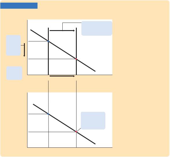
Figure 12-13 shows what happens when the price level falls. Because a lower price level raises the level of real money balances, the LM* curve shifts to the right, as in panel (a). The real exchange rate falls, and the equilibrium level of income rises. The aggregate demand curve summarizes this negative relationship between the price level and the level of income, as shown in panel (b).
Thus, just as the IS–LM model explains the aggregate demand curve in a closed economy, the Mundell–Fleming model explains the aggregate demand curve for a small open economy. In both cases, the aggregate demand curve shows the set of equilibria in the goods and money markets that arise as the price level varies. And in both cases, anything that changes equilibrium income, other than a change in the price level, shifts the aggregate demand curve. Policies and
FIGURE 12-13
Real exchange rate, e
2. ...
lowering e1
the real
exchange
rate ...
e2
(a) The Mundell–Fleming Model
LM*(P1) |
LM*(P2) 1. A fall in the price |
|
level P shifts the LM* |
|
curve to the right, ... |
3. ... and |
|
|
|
IS* |
||
raising |
|
|
|
|||
|
|
|
|
|||
income Y. |
Y1 |
|
Y2 |
Income, output, Y |
||
|
||||||
|
|
|||||
(b) The Aggregate Demand Curve
Price level, P
P1 |
|
4. The AD curve |
||
|
|
|
|
summarizes the |
|
|
|
|
relationship |
|
|
|
|
between P and Y. |
P2 |
|
|
|
AD |
|
|
|||
|
|
|||
|
|
|
|
|
Y1 |
Y2 |
Income, output, Y |
||
Mundell–Fleming as a
Theory of Aggregate Demand Panel (a) shows that when the price level falls, the LM* curve shifts to the right. The equilibrium level of income rises. Panel (b) shows that this negative relationship between P and Y is summarized by the aggregate demand curve.

368 | P A R T I V Business Cycle Theory: The Economy in the Short Run
events that raise income for a given price level shift the aggregate demand curve to the right; policies and events that lower income for a given price level shift the aggregate demand curve to the left.
We can use this diagram to show how the short-run model in this chapter is related to the long-run model in Chapter 5. Figure 12-14 shows the short-run and long-run equilibria. In both panels of the figure, point K describes the shortrun equilibrium, because it assumes a fixed price level. At this equilibrium, the demand for goods and services is too low to keep the economy producing at its natural level. Over time, low demand causes the price level to fall. The fall in the
FIGURE 12-14
(a) The Mundell–Fleming Model
Real exchange |
LM*(P1) |
LM*(P2) |
|
rate, e |
|
||
e1 |
K |
|
|
|
|
|
|
e2 |
|
C |
|
|
|
|
|
|
|
|
IS* |
|
Y1 |
Y |
Income, output, Y |
The Short-Run and Long-Run Equilibria in a Small Open Economy Point K in both panels shows the equilibrium under the Keynesian assumption that the price level is fixed at P1. Point C in both panels shows the equilibrium under the classical assumption that the price level adjusts to maintain − income at its natural level Y .
(b) The Model of Aggregate Supply
and Aggregate Demand
Price level, P
|
LRAS |
|
K |
P1 |
SRAS1 |
P2 |
SRAS2 |
|
C |
|
AD |
YIncome, output, Y