

3.5 MODELING AND ENHANCING THE DATA CAPACITY OF WIRELESS SENSOR NETWORKS |
157 |
Collision avoidance area
Figure 3.22 Another protocol for collision avoidance is simulated. Here, we have eliminated overshoot after collision avoidance using a braking acceleration.
3.5 MODELING AND ENHANCING THE DATA CAPACITY OF WIRELESS SENSOR NETWORKS
Jie Lian, Kshirasagar Naik, and Gordon B. Agnew
Energy conservation is one of the most important design considerations for battery-powered wireless sensors networks (WSNET). Energy constraint in WSNETs limits the total amount of sensed data (data capacity) received by the sink. The data capacity of WSNETs is significantly affected by deployment of sensors and the sink. A major issue, which has not been adequately addressed so far, is the question of how node deployment governs the data capacity and how to improve the total data capacity of WSNETs by using nonuniform
Collision avoidance area
Figure 3.23 In this simulation, we achieve collision avoidance by guiding agents along curves in space, once potential collision is detected.
158 PURPOSEFUL MOBILITY AND NAVIGATION
sensor deployment strategies. We discuss this problem by analyzing the commonly used static model of sensors networks. In the static model, we find that after the lifetime of a sensor network is over, there is a great amount of energy left unused, which can be up to 90% of the total initial energy. This energy waste implies that the potential data capacity can be much larger than the capacity achieved in the static model. To increase the total data capacity, we propose two strategies: a nonuniform energy distribution model and a new routing protocol with a mobile sink. For large and dense WSNETs, both of these strategies can increase the total data capacity by an order of magnitude.
3.5.1 Background Information
A WSNET consists of a set of microsensors deployed within a fixed area. The sensors sense a specific phenomenon in the environment and route the sensed data to a relatively small number of central processing nodes, called sinks. Unlike a mobile ad hoc network (MANET) where bandwidth efficiency and throughput are two important metrics, energy conservation is an important design consideration for WSNETs. This is because all sensors are constrained by battery power. Moreover, since sensor networks generally operate at low data rates, signal interference among neighbors is not much of an issue compared to MANET.
Similar to MANETs, researchers have focused on the medium (media) access control (MAC) and network layer protocols for WSNETs [15, 26, 70–75, 83]. Data aggregation techniques also have been studied in [15, 70, 75, 76]. In fact, all of these focus on increasing the energy efficiency of a WSNET, which is represented by the average energy required to transmit a unit of sensed data to a sink. A commonly used model of WSNETs in those studies is the static model in which homogenous sensors are uniformly distributed in the sensed area with one stationary sink. In the static model, we may observe that sensors close to the sink need to forward more data than sensors far away from the sink. Thus, sensors close to the sink exhaust their energy much faster than other sensors. The extreme case occurs with the direct neighbor sensors of the sink, which deplete their energy first. When all neighbors of the sink exhaust their energy, the sink is disconnected from the network, and the lifetime of the network is over. Therefore, the network data capacity of a static WSNET, which is defined as the total amount of sensed data received by the sink, is limited and is mainly determined by the total energy in the neighbors of the sink. Meanwhile, when the lifetime of a network is over, there is an unknown amount of energy left unused. Therefore, it is useful to find the data capacity and energy utilization of a WSNET.
The studies listed above for WSNETs emphasize an increasing energy efficiency, and, therefore, prolonging the lifetime of WSNETs. If we assume that the sink receives sensed data in a fixed constant speed, the lifetime of a WSNET can be measured by the network data capacity. However, from the above discussion and the results obtained in this section, in the commonly used static model of WSNETs energy efficiency is not the most important factor in WSNET operation. Instead, we will show in this section that proper deployment (i.e., locations) of sensors and the sink and energy distribution of sensors have a positive impact on the lifetime (or the data capacity) of WSNETs.
The contributions of this section are summarized as follows. First, we will develop a mathematical model of static WSNETs with uniformly distributed, homogenous sensors and a single stationary sink; next, we will analyze its performance. Performance of a WSNET is evaluated using three metrics: network data capacity, energy efficiency, and
3.5 MODELING AND ENHANCING THE DATA CAPACITY OF WIRELESS SENSOR NETWORKS |
159 |
energy utilization. Unlike the transport capacity of a wireless network discussed in the literature [77, 78], network data capacity of a sensor network is the total amount of sensed data received by the sink. The main observations from this model are that a significant amount of energy is still left unused after the lifetime of the network is over, and the total data capacity achieved is much smaller than the maximum potential data capacity. For moderate size and large WSNETs, after the lifetime of a network is over, there is a large amount of energy left unused, which can be up to 90% of the total initial energy. These results suggest that the static model is not a good choice for large-scale sensor networks. The main reasons for the inefficient energy utilization are the uniform energy level of all sensors and the stationary sink. Therefore, to increase the total data capacity, we propose a nonuniform energy distribution model and a new routing protocol with mobile sink support. Simulation study shows that these two strategies can improve the total data capacity by an order of magnitude of the data capacity achieved in the static single-sink model.
3.5.2 Basic Assumptions
We focus on large-scale, dense networks with several hundreds to thousands of sensors. For these networks, without any loss of generality, we make the following assumptions:
The network area is a fixed W × H rectangular area with width W and height H . N sensors are randomly placed according to Poisson distribution [81, 82] with density λ sensors per unit area. Hence, N = λWH.
All sensors are homogeneous in the sense that all of them have the same amount of initial energy Ps and the same transmission range rs . Each sensor consumes ps quantity of energy to transmit one bit of data.
The locations of the sensors and the sink remain unchanged in the static model.
The sensed phenomenon is randomly occurred in the network area over time.
The sink has unlimited energy and the same transmission range rs as the sensors.
The energy required to transmit data is much more than the energy consumed by CPU processing, sensing, and data receptions. Thus, only the power consumption of data transmission is considered.
Two sensors or a sensor and the sink are said to be neighbors if they are within the transmission range of each other. The average degree g of a sensor is defined as the average number of neighbors of a sensor. Due to the sensors being randomly distributed with Poisson process, we have
g = λπrs2 |
(3.42) |
To deploy a sensor network with hundreds of nodes connected with high probability, say, 0.95, the average degree is at least 4 [79–81]. We assume that the required average degree is not less than 5 to ensure connectivity. When a node senses the phenomenon, we assume that the node chooses the shortest path (with minimum number of hop count) to forward data toward the sink. We ignore the route maintenance overhead and the reason is explained in Section 3.5.3. Due to the low data rate in WSNETs, we assume that data collisions at the MAC level are negligible.
160 PURPOSEFUL MOBILITY AND NAVIGATION
(0, H ) |
|
|
|
|
(x, y) |
|
Sensors |
|
rs |
|
|
O |
Sink(xc, yc=0) |
(W, 0) |
x |
|
Figure 3.24 Illustration of the SSEP model.
3.5.3 Single Static Sink Edge Placement Model
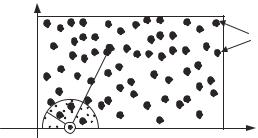
We consider a static model of WSNETs and analyze its data capacity—and energy utilization. In the model, we consider a WSNET with a single stationary sink located on an edge of the rectangular network area. Also, the sink is at least rs distance away from the corners of the network area. This model is referred to as the single static sink edge placement (SSEP) model as illustrated in Figure 3.24. We refer to this kind of a sensor network as an SSEP network.
Due to randomly distributed sensors, the data capacity—of an SSEP network is limited by the total initial energy in the neighbors of the sink. Each bit of sensed data in needs to be forwarded to the sink on a multihop path. Since we assume that the sensed phenomenon is uniformly distributed over time in the network area, the average hop length of all shortest multihop paths can be computed. Using this average hop length, the average energy needed to send one bit of data to the sink can be computed. Therefore, the total energy needed to transmit bits of sensed data to the sink is easily computed. From this utilized energy and the total initial energy, we can obtain the energy utilization ratio in the SSEP model.
3.5.4 SSEP Model Description
In the SSEP model shown in Figure 3.24, we assume that the sink node is located at coordinate (xc, 0) and its location never changes. The reason for using this sink placement model is that in many real situations, the sink cannot move into the sensed area due to some adverse conditions in that area, such as the area being close to a volcano, for example. A network in the SSEP model is determined by six parameters: the area width W , the area height H , the average degree g of sensors, the transmission radius rs , and the location of the sink (xc, yc), where yc = 0.
3.5.5 Critical Region and Network Data Capacity
Definition 3.5.1 The total network data capacity of a WSNET is defined as the total amount of sensed data received by the sink. (It does not include other data such as routing overhead.)
The first critical region, denoted by V1, of the sink is defined as the shaded half circle centered at the sink and with a radius rs in Figure 3.24. It may be noted that V1 contains

3.5 MODELING AND ENHANCING THE DATA CAPACITY OF WIRELESS SENSOR NETWORKS |
161 |
an average of g/2 (half of the degree) sensors. The sink can only receive data from sensors in V1. Thus, the lifetime of the network is over if all sensors in V1 deplete their energy. Since the average total initial energy available in V1 is Ps g/2, where g = λπrs2, and transmission of one bit of data from a sensor in V1 to the sink consumes ps amount of
energy, the average value of the total network data capacity , denoted by , is given as follows:
|
|
1 1 |
|
1 |
|
2 Ps |
(3.43) |
||||
|
|
|
|
||||||||
= |
|
|
Ps g |
|
= |
|
λπrs |
|
|
||
2 |
ps |
2 |
|
ps |
|||||||
In an ideal situation where there is no routing overhead, no collision at the MAC level, and the energy consumed in sensing and computation are negligible compared to data transmissions, the average data capacity can be close to .
3.5.6 Energy Efficiency of a WSNET in the SSEP Model
To calculate the energy utilization of an SSEP network, we need to know the average amount of energy required to transmit one-bit of sensed data along a forwarding path to the sink. This is done by finding the transmission energy efficiency as follows:
Definition 3.5.2 The transmission energy efficiency is defined as the reciprocal of the average amount of energy required to transmit one bit of sensed data along a multihop path from the original sensor to the sink.
A larger value of indicates that less energy is required for data transmission. Since the sensed data should be forwarded to the sink via a multihop path, the smaller the average number of hop counts, the higher the energy efficiency. Therefore, the potential highest energy efficiency can be achieved if sensors use the shortest-hop paths.
To compute , we need to find the average hop count for all shortest-hop paths. However, direct computation of the average hop count is not straightforward for a randomly deployed WSNET. Instead, we use a statistical method as follows. For any given sensor P with many neighbors, P always chooses a neighbor node, which is nearest to the sink, as the next forwarding node. The selected node then follows the same rule to choose the next node, and so on, until the data packet reaches the sink. In general, each forwarding operation reduces the remaining distance from a sensor to the sink by the maximum length, and this length is called the maximum one-hop progress toward the sink. Intuitively, a forwarding path established by this rule is generally the shortest-hop path from P to the sink because the network is dense. The hop count of a shortest-hop path from P to the sink is approximately equal to the distance from P to the sink divided by the average maximum one-hop progress. Therefore, the average hop count of all shortest-hop paths is approximately equal to the average distance to the sink from all sensors divided by the average maximum one-hop progress. Next, we will derive the expressions for the average distance and the average maximum one-hop progress.
Due to the randomly occurring phenomenon in the sensed area, each shortest-hop path has equal probability of being chosen as a forwarding path. For a large and dense network, the problem is equivalent to finding the average distance from all points in the network area to the sink. Assume that the sink is located at (xc, yc). For a given node with coordinate
|
|
|
|
|
(x, y), the distance d from this node to the sink is given by d = |
|
(x − xc)2 + (y − yc)2. |
||
Integrating d over the entire network area, we compute the |
average value of d, denoted by |
|||
|
|
|
|
|
162 PURPOSEFUL MOBILITY AND NAVIGATION
|
3 |
2 |
|
|
|
4 |
|
1 |
|
|
|
5 |
|
(xc, yc) |
|
|
8 |
|
6 |
7 |
|
|
Figure 3.25 Partition of the W × H area.
d, as follows:
|
1 |
W H |
|
|
d = |
- - (x − xc)2 + (y − yc)2 d y d x |
(3.44) |
||
WH |
00
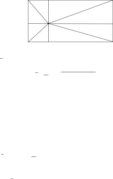
It is difficult to solve (3.44) directly. Instead, we consider the double integral in (3.44) in three-dimensional space. Hence, the double integral is a volume enclosed by the function z = (x − xc)2 + (y − yc)2 and x-y plane with 0 ≤ x ≤ W and 0 ≤ y ≤ H . The entire W−H area can be partitioned into eight triangles as shown in Figure 3.25. For each triangle, we can compute the volume V (x, y) above the triangle as follows, where x and y denote the lengths of the two nondiagonal edges.
|
|
|
0 |
|
|
|
|
|
|
|
|
|
|
|
|
|
|
if x 0 or |
y 0 |
||
V (x, y) |
|
|
|
|
|
|
|
|
|
|
|
|
y |
|
|
|
|
|
|
= |
= |
|
x3 |
|
|
|
2 |
|
2 |
|
|
|
|
2 |
|
2 |
|
||||||
|
= |
|
|
6 |
ln |
y + |
x |
|
+ y |
|
|
− ln (x) + |
x2 |
|
x |
|
+ y |
|
, otherwise |
|
|
The total volume of the double integral is the sum of all volumes of the eight partitioned triangles. Therefore, the solution of (3.44) is the total volume divided by W × H as follows:
d(W, H, xc, yc) = 1 [V (xc, yc) + V (yc, xc) + V (W − xc, yc) + V (yc, W − xc)
WH |
|
+ V (xc, H − yc) + V (H − yc, xc) + V (W − xc, H − yc) |
(3.45) |
+ V (H − yc, W − xc) ] , |
|
where d(W, H, xc, yc) denotes the average distance in the configurations of the area with width W , height H, and the sink location (xc, yc). Since yc = 0 in the SSEP model, the first four addition terms in (3.45) are 0.
The basic idea behind the average maximum one-hop progress has been illustrated in Figure 3.26. In Figure 3.26, P is a sensor node and Q is the sink. Any node on the arc, which is centered at Q and has a radius R = d − z, makes the same forwarding progress z = d − R from P to Q in one hop. When P forwards data to the sink, P always chooses the neighbor node, which makes the maximum progress z, as the next forwarding node. The selected node then follows the same rule to choose the next node, and so on, until the data packet reaches Q. A forwarding path established by this rule is generally the shortest-hop

3.5 MODELING AND ENHANCING THE DATA CAPACITY OF WIRELESS SENSOR NETWORKS |
163 |
|||
|
y |
|
|
|
|
rs |
R = d − z |
|
|
|
P |
Q |
|
|
|
|
|
|
|
|
|
x |
|
|
|
|
B |
|
|
 z
z
d
Figure 3.26 One-hop progress form p to Q.
path from P to Q for a dense network. Next we need to find the expected value of the maximum progress z for a WSNET with average degree g.
There is no simple solution available for this problem. A similar, but not identical, onehop progress problem is discussed in [81]. A solution of the average maximum one-hop progress z has been presented in [82], in which the upper and lower bounds of z are given. These two bounds are tight enough such that the accuracy of z is guaranteed. The average maximum one-hop progress is a function of average degree g, distance d, and radius rs . If we directly use the solution provided in [15], the model will become too complex to analyze. As discussed in [81], if the ratio of d and rs is sufficiently large, z will be a function of the average degree g only, and the influence of d and rs is not significant. This result is supported by a simulation study, which is done as follows.
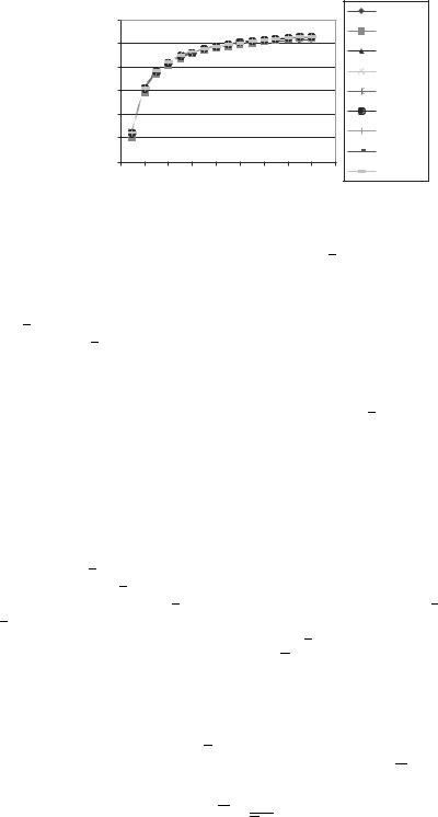
For a particular average degree g, in each round, we randomly generate n nodes based on Poisson distribution with density g within the circle centered at P. Next, we compute the distances from these nodes to Q, choose the node closest to Q, and record its hop progress for this round. We repeat the above three steps for a large number of times and obtain the mean value z. The experimental results are shown in Figure 3.27 for the value of g ranging from 5 to 80. All distances are normalized to transmission radius rs , which is treated as unity. The ratios for data series in Figure 3.27 denote the values of d/rs . All values of z are normalized to rs too. We observe that when both the ratio d/rs and the average degree are greater than 6, z mainly depends on degree g alone. For smaller ratio d/rs and average degree, the differences among all curves are about 10% of the total z.
|
|
1 |
|
|
|
|
|
|
|
|
|
hop |
|
0.9 |
|
|
|
|
|
|
|
|
|
one- |
|
0.8 |
|
|
|
|
|
|
|
|
|
maximum |
progress |
|
|
|
|
|
|
|
|
|
|
0.7 |
|
|
|
|
|
|
|
|
|
||
0.6 |
|
|
|
|
|
|
|
|
|
||
Average |
|
|
|
|
|
|
|
|
|
|
|
|
0.5 |
|
|
|
|
|
|
|
|
|
|
|
|
|
|
|
|
|
|
|
|
|
|
|
|
0.4 |
|
|
|
|
|
|
|
|
|
|
|
0 |
10 |
20 |
30 |
40 |
50 |
60 |
70 |
80 |
90 |
Average degree
 Ratio = 5


 Ratio =10
 Ratio =15
 Ratio = 20
 Ratio = 25
 Ratio = 30
 Ratio = 35


 Ratio = 40
Figure 3.27 Simulation results for the average maximum one-hop progress.
164 PURPOSEFUL MOBILITY AND NAVIGATION
|
|
1 |
|
|
|
|
|
|
|
|
|
Approx |
|
|
|
|
|
|
|
|
|
|
|
Ratio = 5 |
|
hop |
|
0.9 |
|
|
|
|
|
|
|
|
|
|
|
|
|
|
|
|
|
|
|
|
Ratio = 10 |
||
- |
|
|
|
|
|
|
|
|
|
|
|
|
one |
|
|
|
|
|
|
|
|
|
|
|
|
|
0.8 |
|
|
|
|
|
|
|
|
|
Ratio = 15 |
|
maximum |
progress |
|
|
|
|
|
|
|
|
|
||
|
|
|
|
|
|
|
|
|
|
|||
0.7 |
|
|
|
|
|
|
|
|
|
Ratio = 20 |
||
0.6 |
|
|
|
|
|
|
|
|
|
Ratio = 25 |
||
Average |
|
|
|
|
|
|
|
|
|
|
||
|
0.5 |
|
|
|
|
|
|
|
|
|
Ratio = 30 |
|
|
|
|
|
|
|
|
|
|
|
|
||
|
|
|
|
|
|
|
|
|
|
|
Ratio = 35 |
|
|
|
0.4 |
|
|
|
|
|
|
|
|
|
|
|
|
|
|
|
|
|
|
|
|
|
Ratio = 40 |
|
|
|
0 |
10 |
20 |
30 |
40 |
50 |
60 |
70 |
80 |
90 |
Average degree
Figure 3.28 Approximated and simulated average maximum one-hop progress.
From the above discussion, an approximate solution for z is estimated as follows:
|
= 1 − e−1/2√ |
|
− 0.07 − 0.09e(5−g)1/3 |
(3.46) |
z |
g |
where z is normalized to rs and g ≥ 5.
The values of z obtained from (3.46) and from simulation studies are compared in Figure 3.28. The curve labeled “Approx” denotes the approximated data obtained from (3.46). We observe that the approximated data matches very well with the simulated data within the range 10 ≤ d/rs ≤ 40 and 10 ≤ g ≤ 60, which are the most commonly used ranges in real applications. The reader may note that the values of z estimated using (3.46) have an error margin of about 10% if d/rs ≤ 7.
Equation (3.46) has been validated by performing simulation studies on randomly generated sensors networks. In the experiments, we randomly deploy homogeneous sensors in a W × H network area with average degree g. We generated networks with different configurations: The ratio of W/H was varied from 1 to 20; the average degree g was varied from 5 to 80; and the sink locations were changed from the middle of the W edge to a corner of the network area. For those networks, we computed the maximum one-hop progress for each node connecting to the sink and then computed the average maximum one-hop progress z. This simulated average maximum one-hop progress is compared with the calculated progress z based on (3.46). From the simulation results (not shown here), we find that the computed values of z closely match with the simulated values of z. The values of z estimated using (3.46) have an error margin of approximately 10% for g ≤ 7. Hence, Equation (3.46) can be used in estimating the value of z for a given degree g.
Therefore, the approximated average hop count h for all shortest paths is |
|
|||||||||||||||||||
|
|
|
|
|
|
|
|
|
|
|
|
|
|
|
|
|
|
|
|
|
|
|
|
|
d |
|
|
|
|
|
|
|
d |
|
|
|
(3.47) |
||||
|
h ≈ |
|
= |
|
|
|
|
|
|
|
|
|||||||||
|
|
|
|
|
|
|
|
|
|
|
|
|
|
|
||||||
|
rs z |
rs (1 |
− |
e−1/2√g |
− |
0.07 |
− |
0.09e(5−g)1/3) |
||||||||||||
|
|
|
|
|
|
|
|
|
|
|
|
|
|
|
|
|
|
|||
Since sensed data should traverse h hops on average to the sink, and transmission for each hop consume ps amount of energy, the average energy efficiency is
= |
1 |
(3.48) |
h ps